Turning Relational Data Into Graph Visualizations with PuppyGraph and G.V()
In this article we’ll showcase a first of its kind Graph analytics engine that transform and unify your relational data stores into a highly scalable and low-latency graph. I present to you: PuppyGraph!
Introduction
What is PuppyGraph?
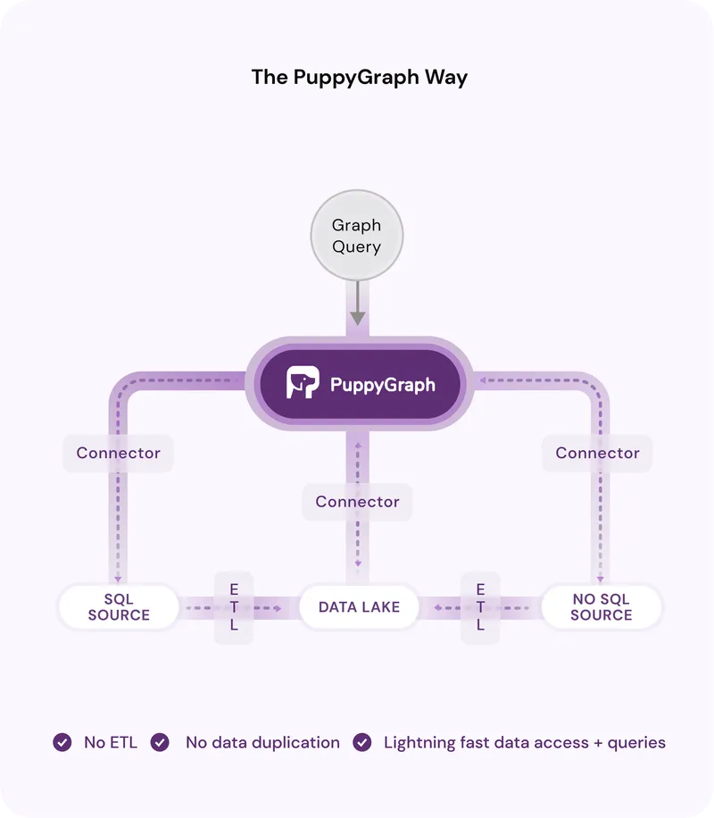
PuppyGraph is a deployable Graph Analytic Engine that aggregates disparate relational data stores into a queryable graph, with zero ETL (Extract, Transform, Load) requirements. It’s plug and play by nature, requiring very little setup or learning: deploy it as a Docker container or AWS AMI, configure your data source and data schema, and you’ve got yourself a fully functional Graph Analytics Engine.
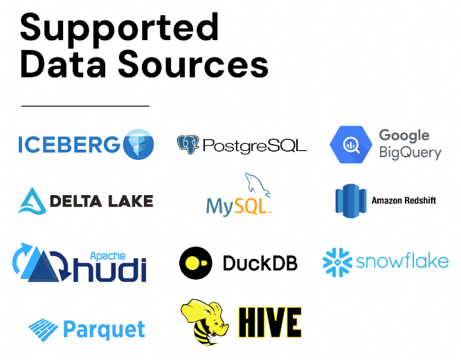
The list of supported data sources is long and growing. At time of writing PuppyGraph supports all of the below sources:
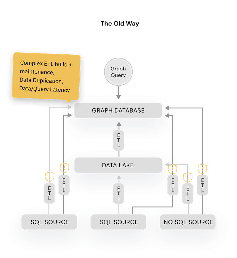
PuppyGraph’s unique selling point is to deliver all the benefits of a traditional graph database deployments without any of the challenges:
- Complex ETL: Graph databases require building time-consuming ETL pipelines with specialized knowledge, delaying data readiness and posing failure risks.
- Scaling challenges: Increasing nodes and edges complicate scaling due to higher computational demands and challenges in horizontal scaling. The interconnected nature of graph data means that adding more hardware does not always translate to linear performance improvements. In fact, it often necessitates a rethinking of the graph model or using more sophisticated scaling techniques.
- Performance difficulties: Traditional graph databases can take hours to run multi-hop queries and struggle beyond 100GB of data.
- Specialized graph-modeling knowledge requirements: Using graph databases demands a foundational understanding of mapping graph theory and logical modeling to an optimal physical data layouts or index. Given that graph databases are less commonly encountered for many engineers compared to relational databases, this lower exposure can act as a considerable barrier to implementing an optimal solution with a traditional graph database.
- Interoperability issues: Tool compatibility between graph databases and SQL is largely lacking. Existing tools for an organization’s databases may not work well with graph databases, leading to the need for new investments in tools and training for integration and usage.
Why does PuppyGraph exist and why is it more performant than a traditional graph database?
Under the hood
- catalogs: This is going to be your list of data sources. A data source consists of a name, credentials, database driver class and jdbc URI
- vertices: this is the translation layer between your database tables and your vertices. Each vertex is mapped from a catalog, a schema and a table. Simply put, a table should map to a vertex, and its columns to vertex properties, with a name and a type. In other words, your columns ARE your vertex properties, and you can pick which ones to include as part of your vertex.
- edges: this is translation layer that leverages the relationships of your relational data, and maps them into edges. Think simple: its (mostly) going to be foreign keys. You can even map attributes to your edges from columns of your related tables.
{
  "catalogs": [
    {
      "name": "postgres_data",
      "type": "postgresql",
      "jdbc": {
        "username": "postgres",
        "password": "postgres123",
        "jdbcUri": "jdbc:postgresql://postgres:5432/postgres",
        "driverClass": "org.postgresql.Driver"
      }
    }
  ],
  "vertices": [
    {
      "label": "Location",
      "mappedTableSource": {
        "catalog": "postgres_data",
        "schema": "supply",
        "table": "locations",
        "metaFields": {
          "id": "id"
        }
      },
      "attributes": [
        {
          "name": "address",
          "type": "String"
        },
        {
          "name": "city",
          "type": "String"
        },
        {
          "name": "country",
          "type": "String"
        },
        {
          "name": "lat",
          "type": "Double"
        },
        {
          "name": "lng",
          "type": "Double"
        }
      ]
    },
    {
      "label": "Customer",
      "mappedTableSource": {
        "catalog": "postgres_data",
        "schema": "supply",
        "table": "customers",
        "metaFields": {
          "id": "id"
        }
      },
      "attributes": [
        {
          "name": "customername",
          "type": "String"
        },
        {
          "name": "city",
          "type": "String"
        }
      ]
    }
  ],
  "edges": [
    {
      "label": "CustomerLocation",
      "mappedTableSource": {
        "catalog": "postgres_data",
        "schema": "supply",
        "table": "customers",
        "metaFields": {
          "id": "id",
          "from": "id",
          "to": "location_id"
        }
      },
      "from": "Customer",
      "to": "Location"
    }
  ]
}
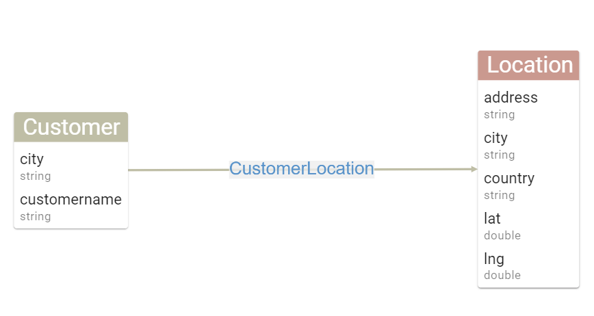
And there you have it! The schema file below would result in the following Graph data schema:
Now that we’ve covered the theory, let’s jump to practice with a step by step guide to create, configure and query your first Graph Analytics Engine using PuppyGraph and G.V().
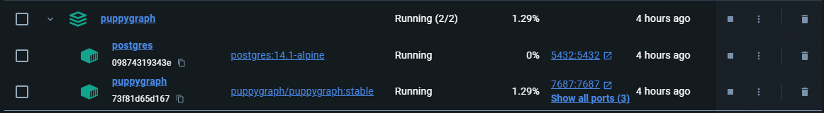
Setting up your first PuppyGraph container
version: "3"
services:
  puppygraph:
    image: puppygraph/puppygraph:stable
    pull_policy: always
    container_name: puppygraph
    environment:
      - PUPPYGRAPH_USERNAME=puppygraph
      - PUPPYGRAPH_PASSWORD=puppygraph123
    networks:
      postgres_net:
    ports:
      - "8081:8081"
      - "8182:8182"
      - "7687:7687"
  postgres:
    image: postgres:14.1-alpine
    container_name: postgres
    environment:
      - POSTGRES_USER=postgres
      - POSTGRES_PASSWORD=postgres123
    networks:
      postgres_net:
    ports:
      - "5432:5432"
    volumes:
      - ./postgres-data:/var/lib/postgresql/data
      - ./csv_data:/tmp/csv_data:ro
      - ./postgres-schema.sql:/tmp/postgres-schema.sql
networks:
  postgres_net:
    name: puppy-postgres
create schema supply;
create table supply.customers (id bigint, customername text, city text, state text, location_id bigint);
COPY supply.customers FROM '/tmp/csv_data/customers.csv' delimiter ',' CSV HEADER;

create table supply.distance (id bigint, from_loc_id bigint, to_loc_id bigint, distance double precision);
COPY supply.distances FROM '/tmp/csv_data/distance.csv' delimiter ',' CSV HEADER;
create table supply.factory (id bigint, factoryname text, locationid bigint);
COPY supply.factory FROM '/tmp/csv_data/factory.csv' delimiter ',' CSV HEADER;

create table supply.inventory (id bigint, productid bigint, locationid bigint, quantity bigint, lastupdated timestamp);
COPY supply.inventory FROM '/tmp/csv_data/inventory.csv' delimiter ',' CSV HEADER;

create table supply.locations (id bigint, address text, city text, country text, lat double precision, lng double precision);
COPY supply.locations FROM '/tmp/csv_data/locations.csv' delimiter ',' CSV HEADER;

create table supply.materialfactory (id bigint, material_id bigint, factory_id bigint);
COPY supply.materialfactory FROM '/tmp/csv_data/materialfactory.csv' delimiter ',' CSV HEADER;

create table supply.materialinventory (id bigint, materialid bigint, locationid bigint, quantity bigint, lastupdated timestamp);
COPY supply.materialinventory FROM '/tmp/csv_data/materialinventory.csv' delimiter ',' CSV HEADER;

create table supply.materialorders (id bigint, materialid bigint, factoryid bigint, quantity bigint, orderdate timestamp,
expectedarrivaldate timestamp, status text);
COPY supply.materialorders FROM '/tmp/csv_data/materialorders.csv' delimiter ',' CSV HEADER;

create table supply.materials (id bigint, materialname text);
COPY supply.materials FROM '/tmp/csv_data/materials.csv' delimiter ',' CSV HEADER;

create table supply.productcomposition (id bigint, productid bigint, materialid bigint, quantity bigint);
COPY supply.productcomposition FROM '/tmp/csv_data/productcomposition.csv' delimiter ',' CSV HEADER;

create table supply.products (id bigint, productname text, price double precision);
COPY supply.products FROM '/tmp/csv_data/products.csv' delimiter ',' CSV HEADER;

create table supply.productsales (id bigint, productid bigint, customerid bigint, quantity bigint,
saledate timestamp, totalprice double precision);
COPY supply.productsales FROM '/tmp/csv_data/productsales.csv' delimiter ',' CSV HEADER;

create table supply.productshipment (id bigint, productid bigint, fromlocationid bigint, tolocationid bigint,
quantity bigint, shipmentdate timestamp, expectedarrivaldate timestamp, status text);
COPY supply.productshipment FROM '/tmp/csv_data/productshipment.csv' delimiter ',' CSV HEADER;
/csv_data
            customers.csv
            distance.csv
            factory.csv
            inventory.csv
            locations.csv
            materialfactory.csv
            materialorders.csv
            materials.csv
            productcomposition.csv
            products.csv
            productsales.csv
            productshipment.csv
docker-compose-puppygraph.yaml
postgres-schema.sql
docker compose -f puppygraph/docker-compose-puppygraph.yaml up
Loading Relational Data and Turning it into a Graph
docker exec -it postgres psql -h postgres -U postgres
\i /tmp/postgres-schema.sql
Then, head on over to localhost:8081 to access the PuppyGraph console. You’ll be prompted to sign in. Enter the following credentials and click Sign In:
Username: puppygraph
Password: puppygraph123
After that, you’ll be presented with a screen with an option to upload your Graph Data Schema. Download our pre-made graph data schema configuration file here, click Choose File, then Upload. PuppyGraph will perform some checks and in just a minute you should be presented with the following on your screen:
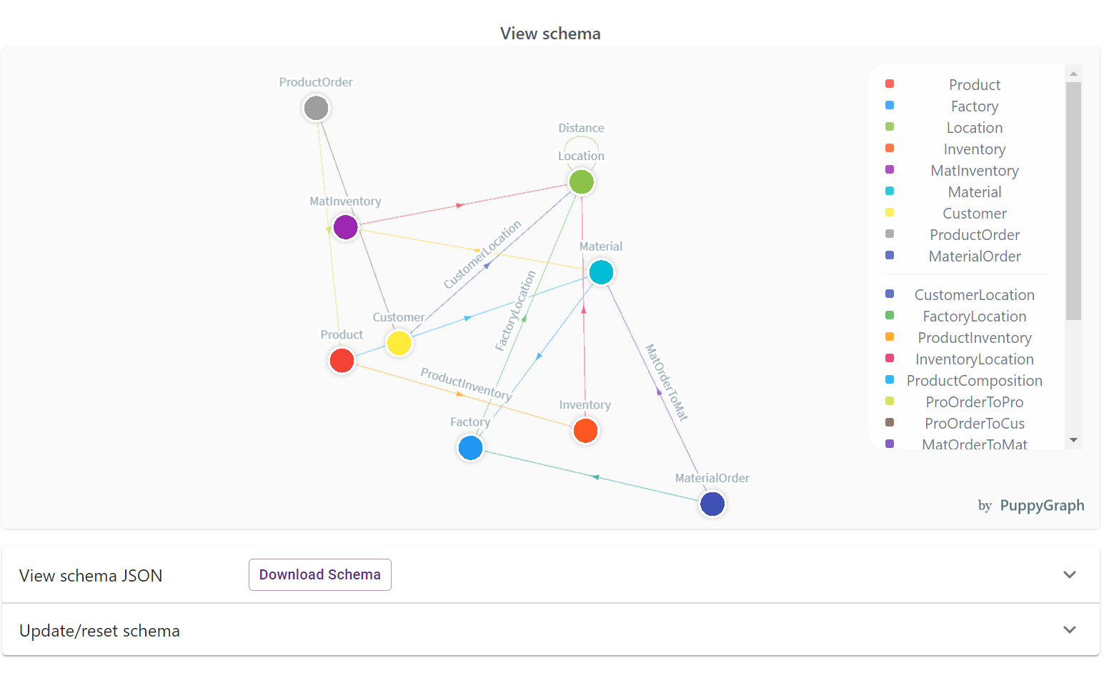
Your PuppyGraph instance is now ready to be queried with G.V() (or using PuppyGraph’s internal tooling)!
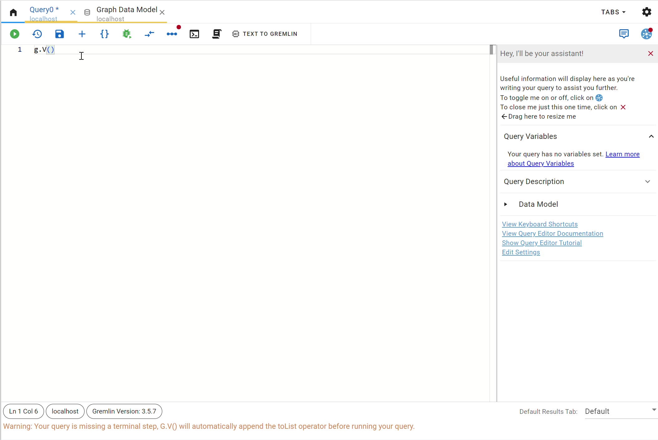
Connecting G.V() to PuppyGraph
Getting insights from your shiny new PuppyGraph instance with G.V()
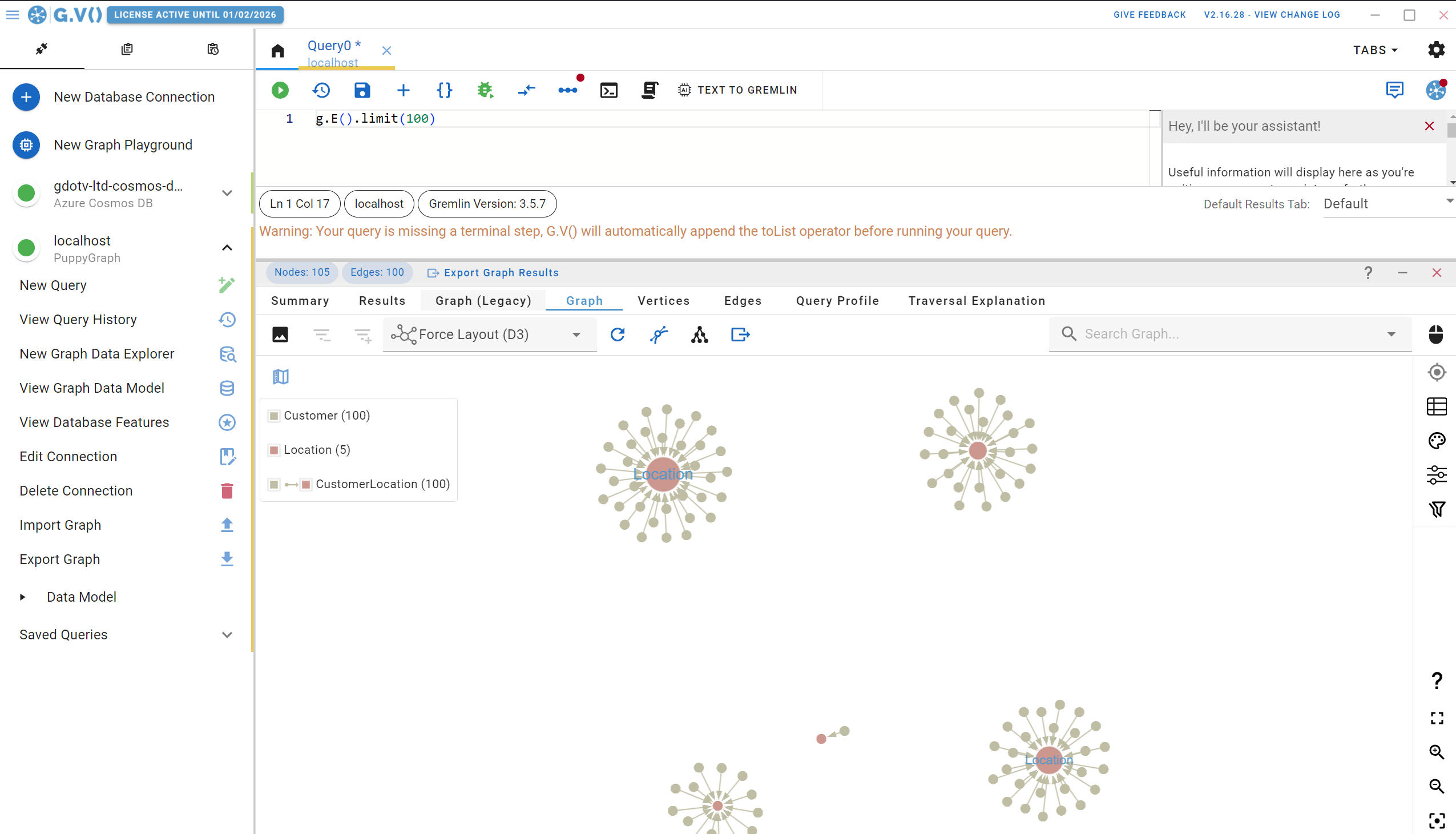
There’s a lot going on in this screen and we’ll come back to that. For now, let’s check out the Entity Relationships diagram G.V() has created for your PuppyGraph data schema. On the left handside, click on View Graph Data Model, and you’ll be presented with the following:
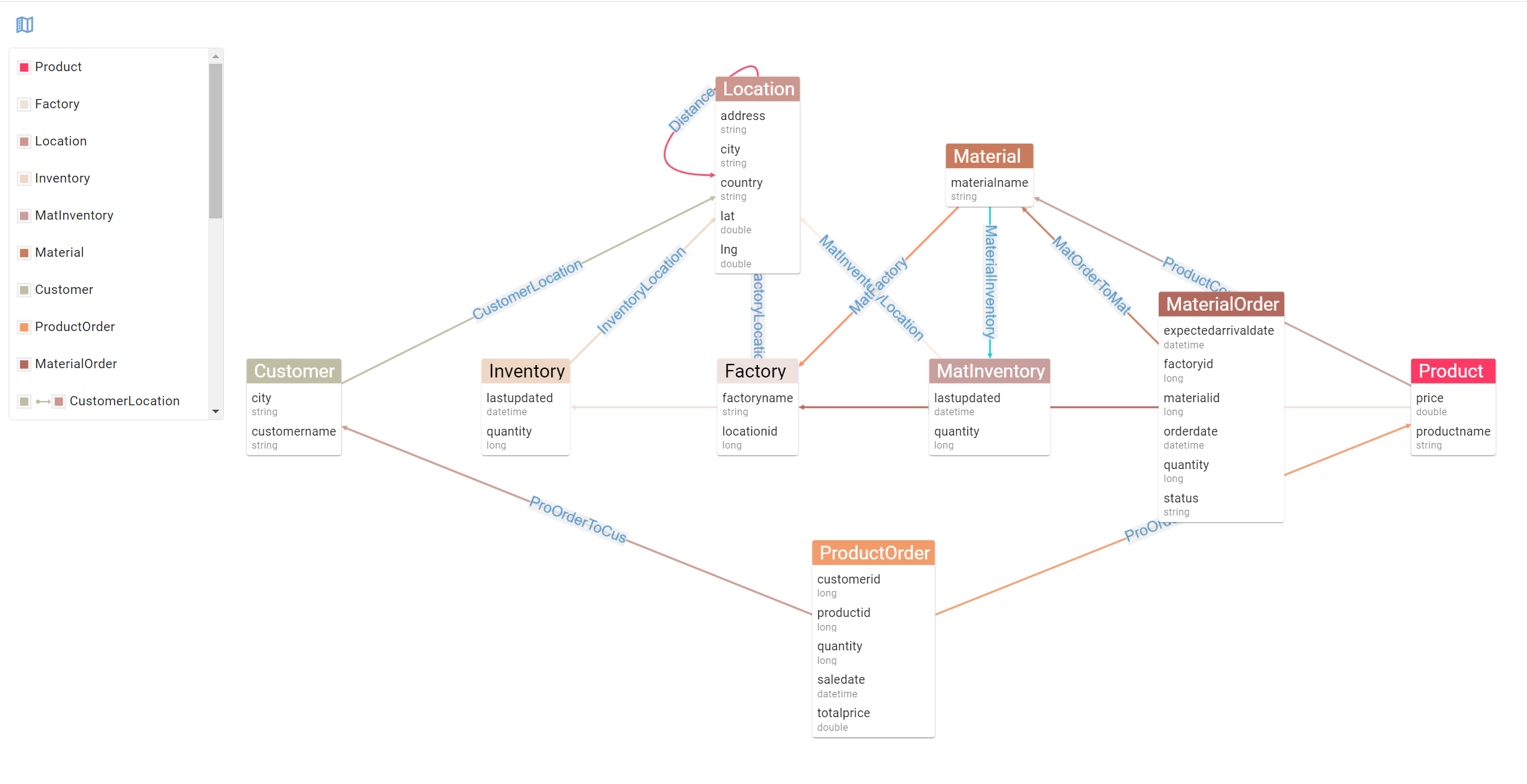
The Entity Relationship diagram G.V() provides gives you an easy way to inspect the structure of your data. This becomes especially useful when mixing multiple data sources in your PuppyGraph data schema as the resulting schema would be different from the individual data models of your data sources. Anyway, the added benefit of G.V() knowing your data schema is that it can also use it to power a whole bunch of features, such as smart autocomplete suggestions when writing queries, or graph stylesheets to customise the look and feel or your displays.
What’s important here is to realise what huge benefits a graph structure brings to your relational data. Let’s take a real life example applied to this dataset and compare how a graph query would perform against a normal SQL query. The dataset we’re using here is a supply chain use case. Unfortunately sometimes in a supply chain, a material can be faulty and lead to downstream impact to our customers.
Let’s say as an example that a Factory has been producing faulty materials and that we need to inform impacted customers of a product recall. To visualise how we might solve this querying problem, let’s filter down our data model to display the relevant entities and relationships we should leverage to get the right query running:
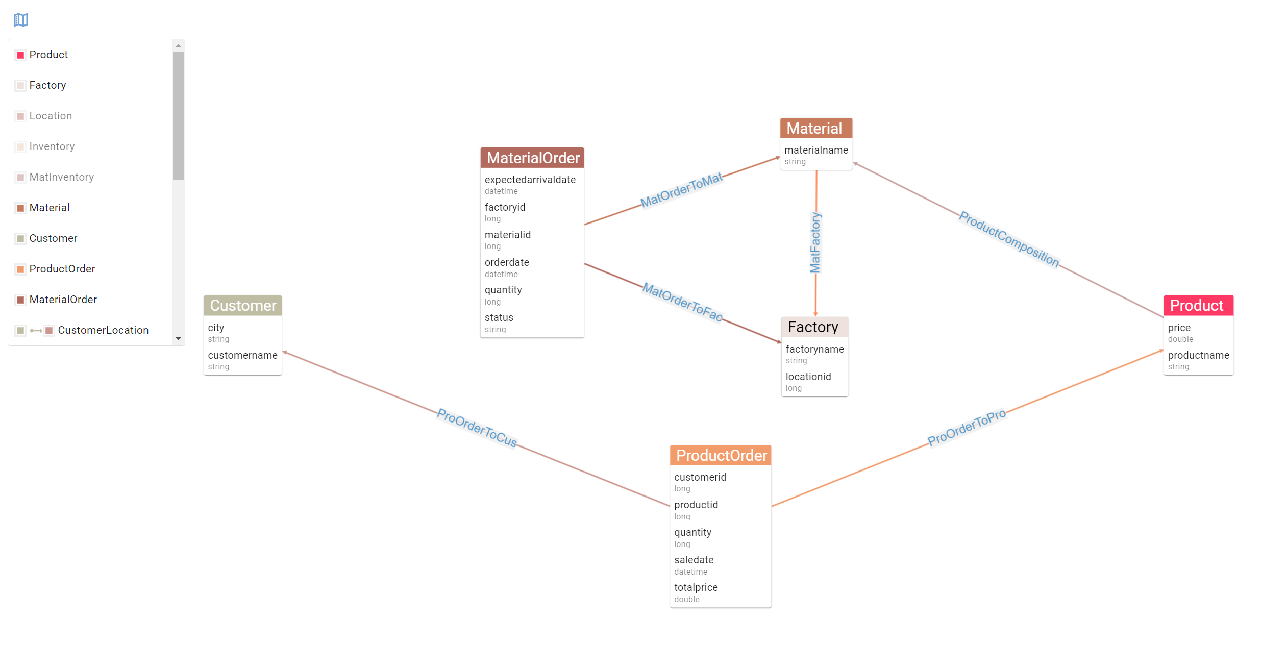
Using this view allows use to see the path to follow from Factory to Customer. This concept of traversing a path in our data from a point A (a factory putting out faulting materials) to point B (our impacted customers) is fundamental in a graph database. Crucially, this is exactly the type of problems graph analytics engine are built to solve. In an SQL world, this would be a very convoluted query: a Factory joins to a Material which joins to a Product which joins to a ProductOrder which joins to a Customer. Yeesh.
Using the Gremlin querying language however, this becomes a much simpler query. Remember that unlike relational databases, where we select and aggregate the data to get to an answer, here we are merely traversing our data. Think of it as tracing the steps of our Materials from Factory all the way to Customer. To write our query, we will pick “Factory 46” as our culprit, and design our query step by step back to our customers.
In Gremlin, we are therefore picking the vertex with label “Factory” and factoryname “Factory 46”, as follows:
g.V().has("Factory", "name", "Factory 46")
This is our starting point in the query, our “Point A”. Next, we simply follow the relationships displayed in our Entity Relationship diagram leading to our unlucky Customers.
To get the materials produced by the factory, represented as the MatFactory relationship going out of Material into Factory, we simply add the following step to our query:
g.V().has("Factory", "name", "Factory 46".in("MatFactory")
You should start seeing where this is going. Following this logic, let’s get all the way to our Customers:
g.V().has("Factory", "name", "Factory 46").in("MatFactory").in("ProductComposition").in("ProOrderToPro").out("ProOrderToCus")
And there you have it! This query will return the Customer vertices that have bought products made up of materials manufactured in Factory 46. Best of all, it fits in just one line!
Let’s punch it in G.V() – this will be an opportunity to demonstrate how our query editor’s autocomplete helps you write queries quick and easy:
We can of course create more complex queries to answer more detailed scenarios – for instance, in our example above, we could narrow down to a single faulty material or only recall orders made at a specific date.
The Gremlin querying language offers advanced filtering capabilities and a whole host of features to fit just about any querying scenario. G.V() is there to help you with the process of designing queries by offering smart suggestions, embedded Gremlin documentation, query debugging tools and a whole host of data visualisation options. If you’re interested in a more in depth view of G.V(), check out our documentation, our blog and our website. We also regularly post on upcoming and current developments in the software on Twitter/X and LinkedIn!
Conclusion