Stop Right There: Conducting Fraud Detection with Aerospike Graph

Turns out: Crime is big business (who knew?). Fraud in particular has always been a quick and dirty way to pennies into pounds.

That’s why one of the oldest graph database use cases in the book has always been fraud detection. Every bank and financial services company needs to detect fraudulent transactions accurately and fast, and detecting the complex nature — and distinct visual patterns – of fraud is something graphs are uniquely suited for.

In this blog post, we’ll analyze some banking data using Aerospike Graph and G.V() to complete some straightforward fraud detection.

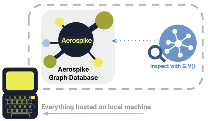
Aerospike Graph is a high-performance graph database that brings the power of graph processing to enterprise scale. It’s powered by the proven performance, scalability, and reliability of the Aerospike Database. Built on the open-source Apache TinkerPop™ framework, it supports the Gremlin query language – giving developers a familiar and flexible way to traverse and manipulate graph data.

Even better, G.V() works natively with Aerospike Graph – helping you query, explore, and analyze connected data at unprecedented scale and speed.

This demonstration is built on top of Aerospike’s own fraud detection demo, which you can find here on GitHub. We’ll see how they define suspicious transactions and how Aerospike implements real-time fraud detection. You’ll also learn how to query the results with Gremlin. Finally, we’ll use a few of G.V()’s own tools to maximize your data exploration.

Here we go!

Getting Set Up with Aerospike & G.V()

Your first step is to get set up with both the Aerospike demo and G.V().

Aerospike Graph will manage and store the graph data itself, and G.V() will visualize the results – helping you see how your queries traverse and connect the data.

Go ahead and follow the setup instructions to get the demo installed on your machine. This consists of cloning the GitHub repo and running the run_app.sh shell script. (Note that you will need Docker installed to run the container!)

The demo has both a backend and front-end functionality. The main backend is currently based on Python and FastAPI, but this will be transitioning soon to a Java backend with Springboot. The frontend operates via Next.js and Tailwind CSS. Today, we’ll focus on the Pythonic backend, but the principles here will carry over to the update to Java, so make sure to check that out. Keep an eye out for a future post about the frontend as well!

Finally, if you don’t already have G.V() installed, head on over to the download portal.

Getting connected to G.V() is straightforward. All you need to do is navigate to New Graph Connection and the Aerospike graph database will be available via localhost on port 8182. See the pic below for an example. Connecting takes only seconds!

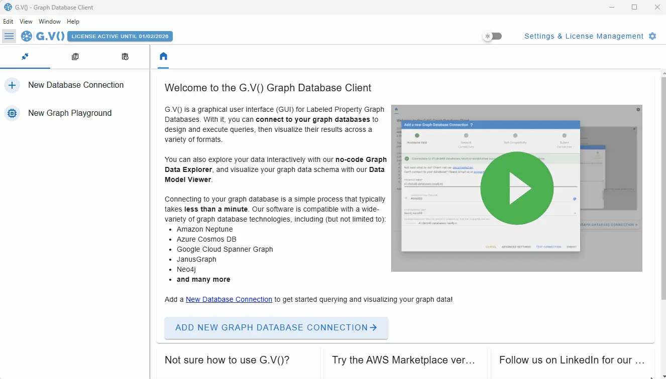Adding a new graph database connection to Aerospike Graph in G.V()

Examining the Data Model

Before we jump straight into exploring the database, let’s review the data schema to understand the structure and relationships in our graph.

What we’ve just set up is a graph-driven real-time fraud detection system. You can find Aerospike’s own intended data model here. (Alternatively, you can find the updated Java version here). Note that the Aerospike demo is still in development, and some components are still under construction or may move around.

For the sake of this demo, we’ll use an abbreviated form of the data model. In this dataset there are just three primary kinds of node (User, Account and Devices) and three types of edges (OWNS, USES and TRANSACTION).

That means that we won’t use FraudResults or Transaction nodes. In our model, transactions are edges only.

This gives us a relatively simple data model that looks like this:

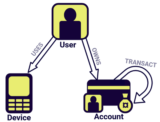Our basic fraud detection data model

So we expect our database to describe a series of User nodes associated with Device and Account nodes corresponding to the accounts and devices that each individual customer owns. Further, we expect some of these Account nodes to be connected via financial transactions.

Note that Account and Device nodes possess the fraud_flag property. We’ll see later on that this is key to how we will conduct fraud analysis in this demo.

Visualizing Your Graph in G.V()

Once you’ve connected to your graph via G.V(), you can instantly visualize the graph via a Gremlin query like g.E().limit(1000):

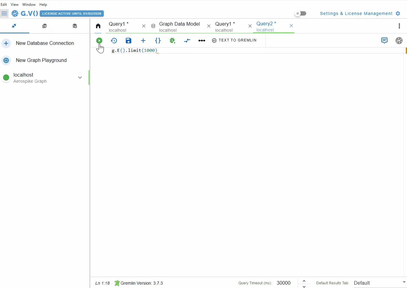Visualizing a Gremlin query in G.V() of our fraud detection dataset

As you can see above, this query produces a number of User, Account and Device nodes, as we expected!

For an overall view of your graph schema, you can click on View Graph Data Model to see the data model:

Examining your graph data model in G.V()

You might notice right away that something is missing. The default graph contains no Transaction edges! What’s going on?

Well, this is actually expected. You’ve initialized the graph in its starting state, as if all our customers have made accounts, but no transactions have actually happened yet. This is actually ideal for our purposes, because we want to do real-time fraud detection, i.e., we want to assess transactions as they happen! We won’t be able to do that if all the transactions already exist.

Before we do that though, let’s take a little extra time to explore the existing data in G.V(), just to see what we’re working with. G.V() is fully compatible with the Gremlin query language, so you can query your graph in the normal way using G.V()’s query editor.

You can look at an example of a node by running the following Gremlin query to look at the user with the name ‘Mariah Greer’:

g.V().hasLabel('user').has('name', 'Mariah Greer').outE()

From here you can customize your graph style sheet to modify the appearance of your graph visualization however you like. This includes modifying the colors and traits of your nodes and edges, as well as labelling them according to whatever properties you desire.

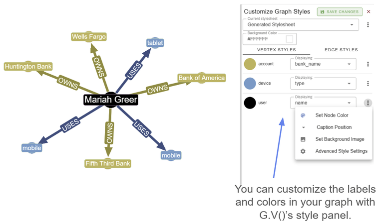Customizing your graph style sheets in G.V() is simple and straightforward

You can also play with different layouts to change the appearance of your graph!

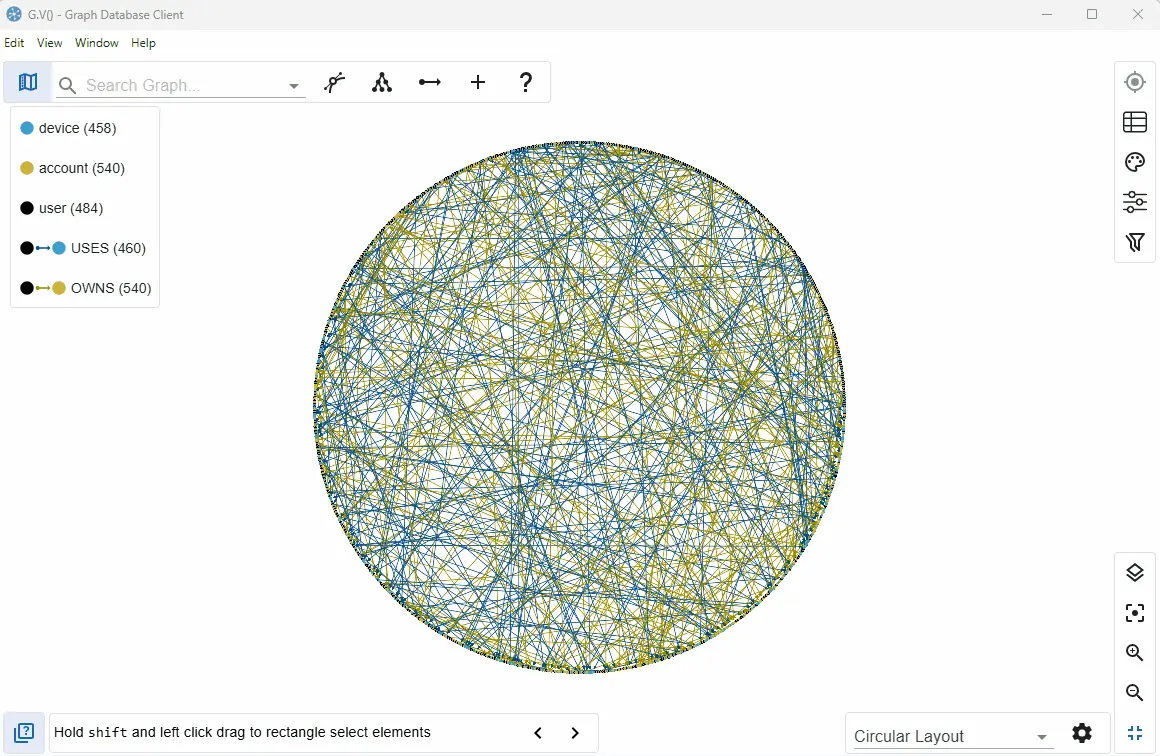You have a lot of graph visualization options in G.V()

That means the next step is to add some transactions!

Making Transactions

The Aerospike Graph demo includes a wealth of useful code for us to play with. As we mentioned previously, the demo will soon be transitioning to a Java backend, so you should keep an eye on that branch for the most up-to-date changes. That version still will follow similar principles to the current Python backend though, which is what we’ll stick to for now.

In the Python version, the main.py script within the /backend folder contains a number of useful functions that will help you do a little preliminary analysis. Begin by opening an interactive IPython session and running this script:

%run main.py

Next up we want to make sure our graph connection is actually set up, so we use the connect() function attached to our graph_service.

In [-]: graph_service.connect()
Out[-]: True

We’re now ready to operate our graph!

Just to make sure that there really are no transactions in our graph before we start, you can run the get_transaction_stats() functions and should get the result that there are zero transactions in the graph.

In [-]:  get_transaction_stats()
Out[-]: {'total_txns': 0, 'total_blocked': 0, 'total_review': 0, 'total_clean': 0}

Let’s generate a transaction. You can do this in two ways. The first is to randomly generate a transaction using the generate_random_transaction() function. This will pick two accounts at random and generate a transfer amount.

You can also manually create a transaction. Just to make sure that everything is working correctly, we’ll start by manually creating a transaction between Mariah Greer (with account id ‘A511101’) and another user, Emily Williams (account id = ‘A644404’), using the following command:

In [-]: create_manual_transaction(from_account_id='A511101', to_account_id='A644404', amount=15000, transaction_type='transfer')
Out[-]: {'message': 'Transaction created successfully'}

It would be nice to visualize this transaction and make sure it was actually added to the database. This is a great time to use the G.V() Data Explorer. You can find this on the left side panel. From here, you can search for User nodes that own Account nodes, which are connected via transaction edges to other Account nodes owned by User nodes.

Since you’ve only added one transaction, it will be easy to find, so this is already plenty of information. But, if you wanted, you could narrow down the search further by applying an additional filter to look for User nodes that have a name exactly matching ‘Mariah Greer.’

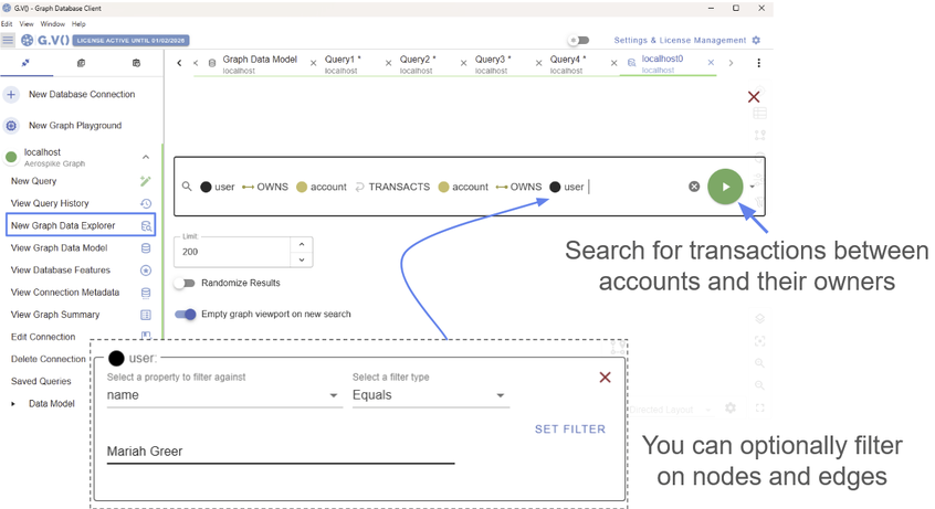
The G.V() Data Explorer lets you search and filter on different levels of detail

Feel free to play around with the filters!

This request should return the transaction we’re interested in, no problem. So you should (hopefully) see that your transaction was added successfully!

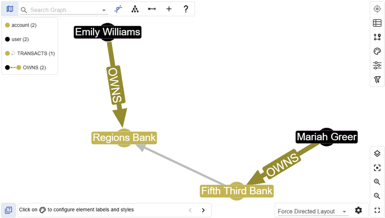
Our potentially fraudulent transaction visualized in G.V()

We can also see our new transaction in G.V() with an appropriate Gremlin query:

g.V().hasLabel('user').has('name', 'Mariah Greer').outE().inV().outE().inV().inE().path()

If you revisit the Data Model, you should also see that a transaction edge has now been added!

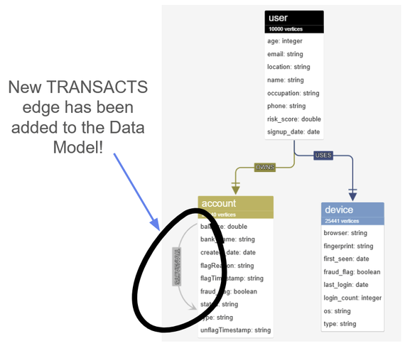
The updated data model now shows a new TRANSACT edge

Examining Flagged Transactions

Okay, everything is working correctly, so let’s create several more transactions using generate_random_transaction()

Create as many as you like. If you do that, then run the get_transaction_stats() function, you should see something like:

In [-]:  get_transaction_stats()
Out[-]: {'total_txns': 30, 'total_blocked': 7, 'total_review': 3, 'total_clean': 20}

It looks like the transactions have already been evaluated! Some have been marked ‘clean’, others are under review, and some have been blocked. What happened?

Well, it turns out that the fraud detection has already been running this entire time! Whenever we create a new transaction, the demo script runs fraud_service.run_fraud_detection() function on these new transactions as part of the function creation process itself. This subjects the transaction to a few checks immediately. This is what is meant by real-time fraud detection, the transaction is evaluated before it even goes through!

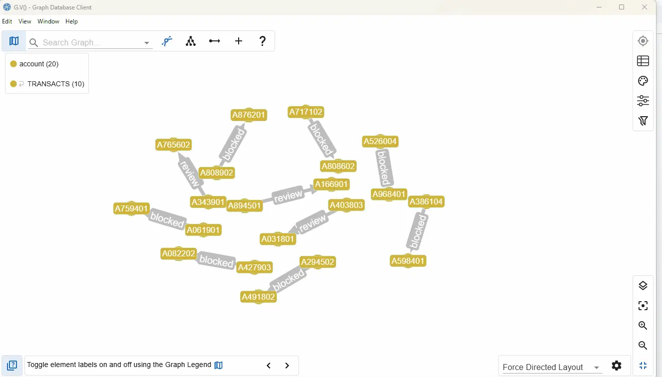
You can use a simple Gremlin query in G.V() to view all the transactions that have a fraud status:

g.E().hasLabel("TRANSACTS").has("is_fraud", true)

Or we could once again use the G.V() Data Explorer:

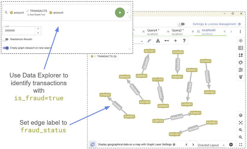
Using the G.V() Data Explorer to find fraudulent transactions

You can identify the Account nodes by their unique ID, then label the TRANSACTS edges by their fraud_status, therefore identifying at a glance which transactions are in review, and which have been blocked.

If we want more information on any particular edge, we just need to click to see the full list of properties. For example, here is an animation taking a closer look at the reason why each transaction was flagged:

Drilling down to view the properties in our graph visualization

Of course, you can also extract all the equivalent edge information within your terminal in a Pythonic way. You could, for example, compile all the properties of the flagged transactions:

In [-]: flagged_transactions = graph_service.client.E().has_label("TRANSACTS").has("fraud_status").to_list()

In [-]: for transaction in flagged_transactions:
     props.append(graph_service.client.E(transaction).value_map().next())

You can then extract the properties of any given transaction to learn more about why it was flagged:

In [-]: props[0]
Out [-]: {'amount': 5551.65,
 'currency': 'USD',
 'details':
[
'{  "flagged_connections":
[{"account_id": "A759401", "role": "receiver", "fraud_score": 100}],
"detection_time": "2025-10-01T15:01:12.946991",
"fraud_score": 100,
"reason": "Connected to 1 flagged account(s) - \'direct fraud\'", "rule": "RT1_SingleLevelFlaggedAccountRule"
}',
  '{   "flagged_connections":
[{"account_id": "A759401", "role": "sender_txn_partner", "fraud_score": 75},
{"account_id": "A759401", "role": "receiver_txn_partner", "fraud_score": 75}],
"total_connections": 2,
"detection_time": "2025-10-01T15:01:12.997177",
"fraud_score": 85,
"reason": "Connected to 2 flagged account(s) - transaction partners", "rule": "RT2_MultiLevelFlaggedAccountRule"
}'
],
 'eval_timestamp': '2025-10-01T15:01:13.059113',
 'fraud_score': 100,
 'fraud_status': 'blocked',
 'gen_type': 'AUTO',
 'is_fraud': True,
 'location': 'Long Beach, California',
 'method': 'electronic_transfer',
 'status': 'completed',
 'timestamp': '2025-10-01T15:01:12.913133',
 'txn_id': '85a6c546-bdb1-4f4c-9527-39e7cd643169',
 'type': 'transfer'}

The best approach depends on your objective and application. The Pythonic approach is more repeatable and integrates better into a more sophisticated pipeline, but the G.V() approach is better for at-a-glance data visualization.

Going Deeper with Fraud Detection

But how did the Aerospike script actually know which transactions to flag for fraud? This is something else you can explore in G.V().

In the current iteration of the fraud_detection script, there are three real-time fraud checks that this function performs:

• Does the TRANSACT edge directly connect to an Account node that has been flagged as suspicious?
• Does the TRANSACT edge connect at least one Account node which is also connected (via an OWNS edge) to a User node that has been flagged as suspicious?
• Does the TRANSACT edge connect at least one Account node which is also connected (via OWNS and USES edges) to a Device node that has been flagged as suspicious?

These are visualized in the following diagram:

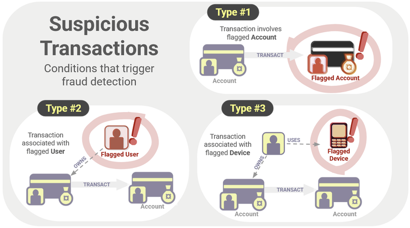
Three types of suspicious transactions that trigger fraud detection in our graph

Whether a node is flagged as suspicious is contained within the fraud_flag property. For now, let’s just consider the first type of suspicious transaction (Type #1: Transactions involving flagged Account nodes). In this case, you can actually manually flag and unflag accounts ourselves, and see the result in G.V().

We can flag an account using the flag_account(account_id, reason) function.

In [-]: asyncio.run(flag_account(account_id = 'A526004', reason='Testing'))
Out[-]:
{'message': 'Account A526004 flagged successfully',
 'account_id': 'A526004',
 'reason': 'Testing',
 'timestamp': '2025-10-06T15:28:27.024966'}

We can unflag the same account using the unflag(account_id) function.

In [-]: asyncio.run(unflag_account(account_id = 'A526004'))
Out[-]:
{'message': 'Account A526004 unflagged successfully',
 'account_id': 'A526004',
 'timestamp': '2025-10-06T15:35:07.038005'}

Each time you flag and unflag the account, check that this node is behaving as you expect! You can look for it using the following Gremlin command in G.V():

g.V().hasLabel('account').hasId('A526004')

You can then view all the properties of this node in G.V()’s viewer. The fraud_flag property should accurately tell you whether this account has been flagged or not.

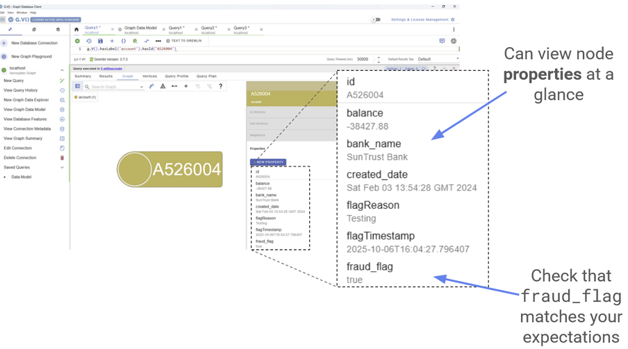
An example of a fraud flag on one of the suspicious accounts

Try doing the same thing for Device and User nodes! (Note that a ‘flagged’ User node is defined as a User connected to a flagged Account.) You should find that all the flagged transactions from the previous section correspond to flagged nodes of some kind. With G.V(), you can see all this information at a glance, allowing for rapid evaluation and response.

Conclusion

In this blog post, we’ve only touched on the very basics of fraud detection.

The Aerospike demo contains a number of further scripts and examples, and is the process of developing more. Part of the demo plan includes implementing further real-time fraud detection techniques, such as detection of supernodes (accounts with a suspiciously high number of connections), time clustering, or ring interactions. There’s also a plan to incorporate batch assessment of transactions. You can investigate for yourself how these kinds of checks might be performed!

Please play around with the dataset yourself, and see what other potential fraud patterns you can identify. Hopefully this demo has shown you that G.V() makes your job easier! Our heartfelt thanks to Aerospike for developing this dataset and associated codebase. Let us know what you think!

Curious to try it out for yourself? Download G.V() today and start visualizing and exploring your connected data with ease.