Getting started with Memgraph and G.V()!
!")
Part 1: Getting started with Memgraph using Lab
Memgraph is a high-performance, open source, in-memory database with low latency. Instead of storing your data on disk or offsite where it needs to be fetched back, Memgraph databases exist entirely within your device’s RAM, greatly accelerating real-time processing speeds and providing you with a lot of scalability. Even better, regular logging and snapshot mechanisms ensure your data is safe even while stored in-memory.
What’s most exciting to us is that Memgraph pairs fantastically with G.V(). Memgraph+G.V() is a classic combination that turns your computer into a formidable tool for analysis and visualization, which is exactly what we’d like to show you today. We’ll first explore how to get started with Memgraph itself and use some of Memgraph’s own built-in visualization options, then we’ll show how G.V() can unlock even more of Memgraph’s potential.
Step 1.1: Starting Memgraph
You can initialize Memgraph by entering the following commands into the appropriate console, depending on your OS:
- On Windows, run
iwr https://windows.memgraph.com | iexin Windows PowerShell - On MacOS, run
curl https://install.memgraph.com | shin the Terminal
Note that you’ll need to have Docker installed and running in the background. For more on Memgraph installation and the various ways to interface with the client, check out Getting started with Memgraph.
Step 1.2: Using the Web Interface & Loading Data
Once Memgraph is initialized, we’ll need to load in some data. Memgraph provides some sample data sets that work great for exploring both Memgraph and G.V(), so let’s connect to Memgraph using their Lab application to explore them.
The web interface can be accessed at http://localhost:3000/login and hitting Connect now.
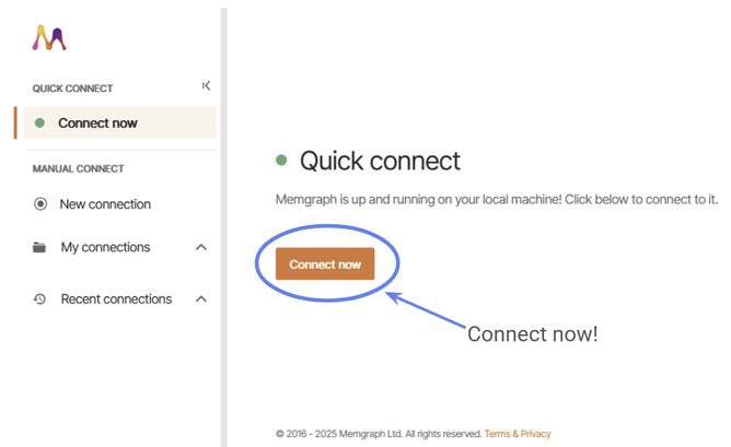
Figure 1: Quick connect to Memgraph Lab.
Within the web application, there are a number of available features. If you have a database ready to go, then you can open it in Memgraph with the Import tab. Alternatively, if you just want to play around (which is what we plan to do!) you can use one of their starter Datasets.
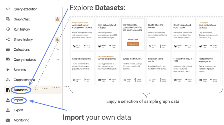
Figure 2: Explore the Memgraph datasets.
To show off the capabilities of Memgraph and G.V(), we’ll start with a reasonably beefy database – let’s try Wikipedia articles – which contains tens of thousands of nodes and hundreds of thousands of edges.
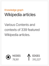
Figure 3: Download the ‘Wikipedia articles’ dataset.
Once you import the data, you’ll be given an option to download a query collection of sample commands customized for this database. Let’s download that as well, and see what’s included.
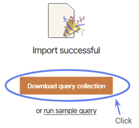
Figure 4: Import the associated query collection.
Now you’ve finished setting up – your sample graph database is now loaded into your computer’s memory. To jump straight into exploration, let’s access the query collection we just downloaded from the Collections tab on the left.
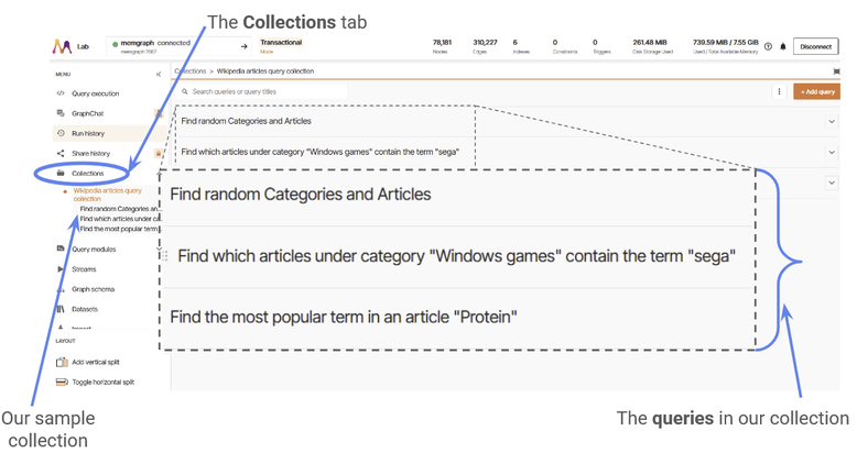
Figure 5: Navigate to the ‘Collections’ tab.
Step 1.3: Running Queries
Let’s try running one and examine the results. We’ll try “Find which articles under category “Windows games” contain the term “sega.” Loading in this query, we can see that queries are written in the Cypher query language. If we click the run query button, we can see there are two results: Sonic the Hedgehog and Dota 2.
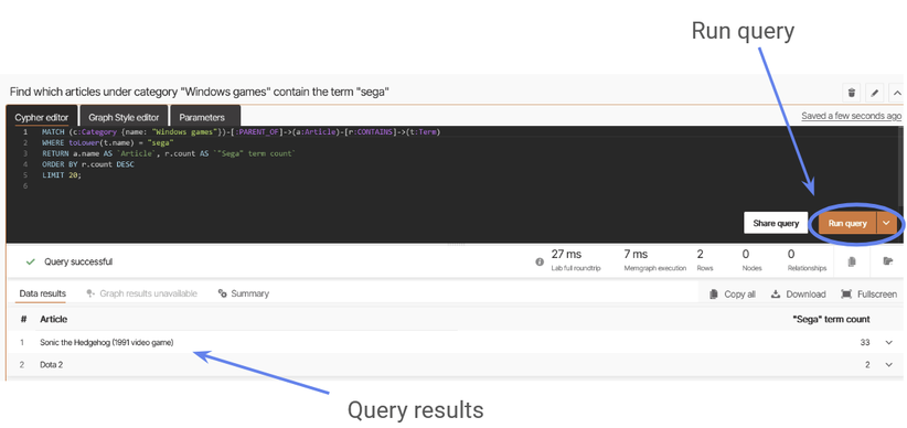
Figure 6: Run a query in Memgraph.
Step 1.4: Visualizing Graphs with Memgraph
Note that for the Wikipedia dataset that we’ve chosen, none of the sample queries demonstrate Memgraph’s graph capabilities by default, because they all return properties rather than the edges and notes themselves.
We can change this by making a slight change to our query:
MATCH (c:Category {name: "Windows games"})-[:PARENT_OF]->(a:Article)-[r:CONTAINS]->(t:Term)WHERE toLower(t.name) = "sega"RETURN a, r, tORDER BY r.count DESCLIMIT 20;
If we run this query, we return the Article, and Term nodes, as well as the CONTAINS relationship. Now we can see the result as a (very simple!) graph.
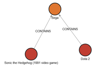
Figure 7: The articles which contain ‘SEGA.’
Let’s use this simple graph to explore how we edit the style or appearance of graphs in Memgraph. We can do this by clicking on System Style.
Here we’re greeted by a Memgraph style sheet, which determines all the rules for how Memgraph will generate visualizations for your graphs. This particular style sheet uses a clever trick to select the colour of its nodes, it defines a COLOR_PALETTE and then iterates over the available colours for each node type. The first two hex codes shown here define the red and orange of the nodes in our graphs.
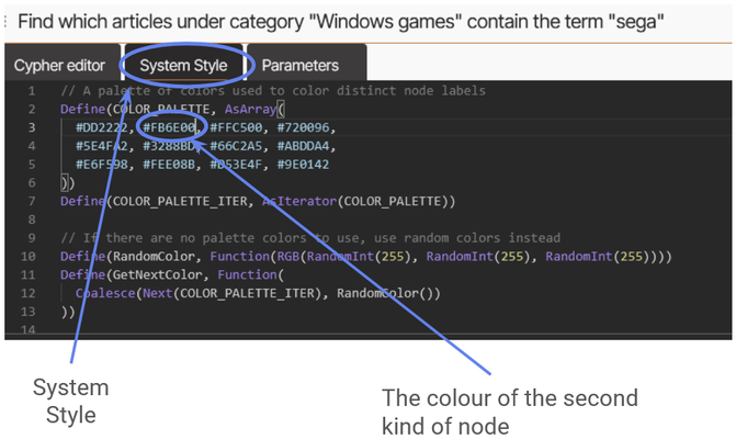
Figure 8: An example Memgraph stylesheet.
The SEGA logo is blue, so let’s change #FB6E00 to #3C5EA2.
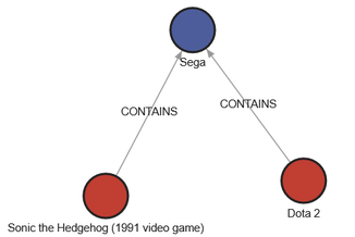
Figure 9: We’ve changed the color of the SEGA node to blue.
By understanding Memgraph’s style sheets, you will have incredible control over your graph’s appearance. Memgraph already have lots and lots information on how you can use style sheets to dynamically generate great visualizations available at the following pages:
- Style your graphs in Memgraph Lab
- Graph Style Script language
- How to Style Your Graph in Memgraph Lab
Memgraph Lab offers a number of other features as well, for example we can revisit queries after we run them in Run History, or view a representation of the graph in Graph Schema. Make sure to consult the Memgraph docs for more information.
Part 2: Introducing G.V() into the Mix
Let’s check out how well Memgraph works in tandem with G.V().
It takes only a second to get connected – once you do, you’ll add a host of new visualization options for your toolkit with no extra effort. G.V() can work as either an alternative or companion to Memgraph Labe – letting you explore all the options at your disposal to select the solution that’s best for your particular project.
Step 2.1: Connecting to Memgraph with G.V()
To get started, just open the G.V() application and look for the Memgraph database with hostname localhost at port 7687. This is Memgraph’s default port.
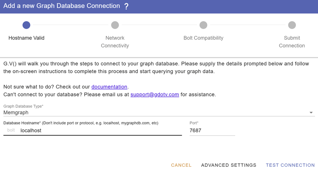
Figure 10: Connect to G.V() instantly.
Hit Test Connection – and you’re done.
(Yes, it’s really that easy!)
Step 2.2: Styling Graphs in G.V()
If we run our SEGA query from before:
MATCH (c:Category {name: "Windows games"})-[:PARENT_OF]->(a:Article)-[r:CONTAINS]->(t:Term)WHERE toLower(t.name) = "sega"RETURN a, r, tORDER BY r.count DESCLIMIT 20;
We can see instantly the same graph is rendered in gdotv:
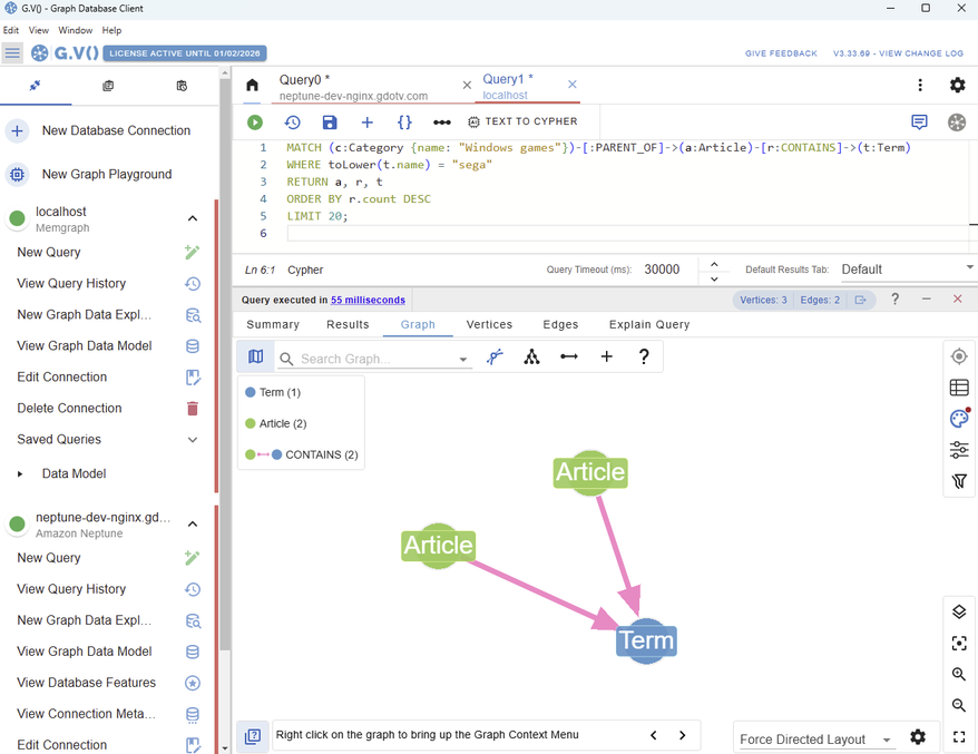
Figure 11: Run the same query in G.V().
You might notice immediately that there are a number of differences from Memgraph, so let’s explore the interface a little to get more comfortable.
Since we’re primarily concerned with visualisation, we’ll focus on the Graph visualization console – which is everything under the Graph tab of our query results.
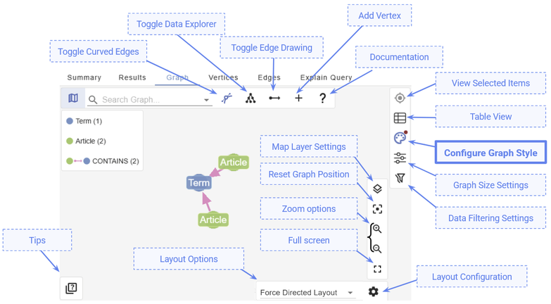
Figure 12: The layout of the G.V() interface.
As you can see, there are a lot of options available to us! For now, let’s go to Configure Graph Style (highlighted in the above diagram). We’d like to see the names of our nodes, just like we did in Memgraph. By default, G.V() shows us the node labels, but we can easily change that by modifying the Caption of any particular node type.
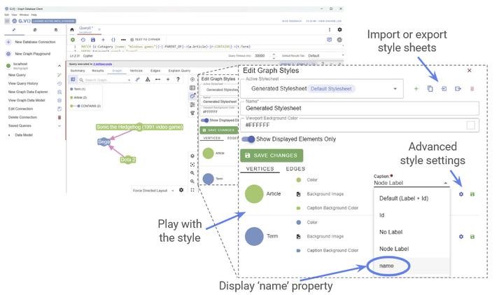
Figure 13: How to modify the style of a graph in G.V().
Not only can we easily set any of our node properties as the caption, we can also modify the visual style of our nodes and edges directly from this interface. A number of options are available to us under Advanced Style Settings, where you can modify the node, edge and caption style to look however you want. You can also modify the layout of the graph under Layout Options, or click and drag nodes by hand.
Right away we can make some fun styles in just a couple of minutes:
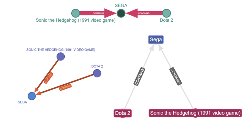
Figure 14: Some example styles you can deploy.
Have a go!
Step 2.3: Viewing Relationships with G.V()
We’d like to probe graphs more complicated than just three nodes. Another thing G.V() lets us do is explore the Data Model at a glance:
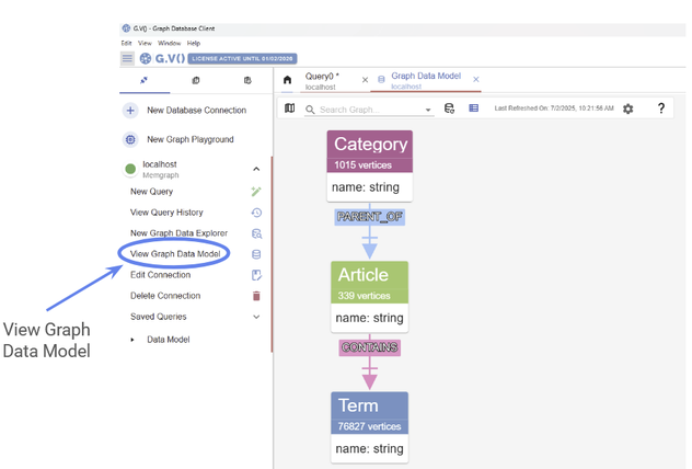
Figure 15: View your data model inside G.V()
We can see that there are three node types – Category, Article and Term.Article nodes refer to wikipedia articles themselves, which contain Term nodes and fall into Category nodes.
Say we wanted to compare two Article nodes. We could compare two famous musicians, Bob Dylan and Devin Townsend. To see at a glance how these nodes look in the dataset, we can, for example, look at the different Category nodes that contain the two musicians:
MATCH (p:Article)<-[e:PARENT_OF]-(c:Category) WHERE p.name = 'Devin Townsend' or p.name = 'Bob Dylan' RETURN p, e, c
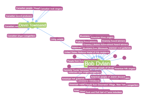
Figure 16: The Category nodes which include Devin Townsend and Bob Dylan.
At a glance, we can see that Bob Dylan and Devin Townsend are categorised quite differently by the dataset! The only Category node we see shared between them is that they are both Living People.
Step 2.4: Modifying Data with G.V()
One reason for the discrepancy is that Bob Dylan has won many more awards than Devin Townsend. That wasn’t what this author set out to show (since I’m a fan of Devin Townsend) but unfortunately data doesn’t always give us results we like.
But it is possible to override data. So, to level the playing field, let’s give Devin all the same awards that Bob Dylan has:
MATCH (p:Article)<-[r:PARENT_OF]-(c:Category) WHERE p.name = 'Bob Dylan' and toLower(c.name) contains 'award'MATCH (d:Article) WHERE d.name = ('Devin Townsend')MERGE (c)-[n_r:PARENT_OF]->(d)SET n_r = properties(r)RETURN 0
Run the query below to check that this worked. Now the result is far more equitable.
MATCH (p:Article)<-[e:PARENT_OF]-(c:Category) WHERE p.name = 'Devin Townsend' or p.name = 'Bob Dylan' RETURN p, e, c
And – actually – if you run the above query in Memgraph, you will see the same result! You can query your database from G.V() and Memgraph simultaneously without conflict.
So you can not only access and visualize data from within G.V(), but you can also make modifications directly within the G.V() console.
Step 2.4: Handling Large Queries with G.V()
Our graphs are still pretty small so far. That’s because there aren’t too many edges between Category and Article nodes in this data set.
To run a bigger query, we could look instead at what Term nodes are contained by the Bob Dylan and Devin Townsend Article nodes:
MATCH (p:Article)-[e:CONTAINS]->(c:Term) WHERE p.name = 'Devin Townsend' or p.name = 'Bob Dylan' RETURN p, e, c LIMIT 100000
This returns ~5,000 edges and 5,000 vertices, which G.V() handles very comfortably.
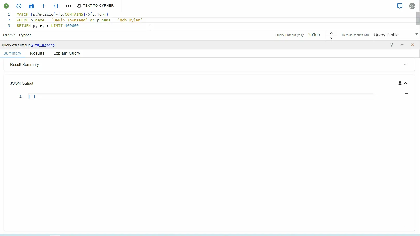
Figure 17: Navigate the terms included in the Bob Dylan and Devin Townsend articles.
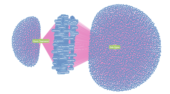
Figure 18: Showing the terms shared by Bob Dylan and Devin Townsend nodes show that Article nodes tend to have relationships with many more Term nodes than Category nodes! We can also see that Bob Dylan seems to have many more adjacent Term nodes – suggesting his Wikipedia article is longer!
Another reason that Bob Dylan (American) and Devin Townsend (Canadian) showed different categories are because many of the Category nodes emphasize nationality. To see how our graph looks with Category, Article and Term nodes, we could look for all of these where the Category node contains the word ‘Canadian’:
MATCH (a:Category)-[b:PARENT_OF]->(p:Article)-[e:CONTAINS]->(c:Term)WHERE a.name contains 'Canadian'RETURN a, b, p, e, c LIMIT 100000
By zooming in on the Term nodes shared by two Article nodes, we can see that (for example) Art Ross and John Cullen are linked by terms like Stanley Cup, Toronto Maple Leafs and Boston Bruins, which reflect the fact that Art Ross and John Cullen are both ice hockey players.
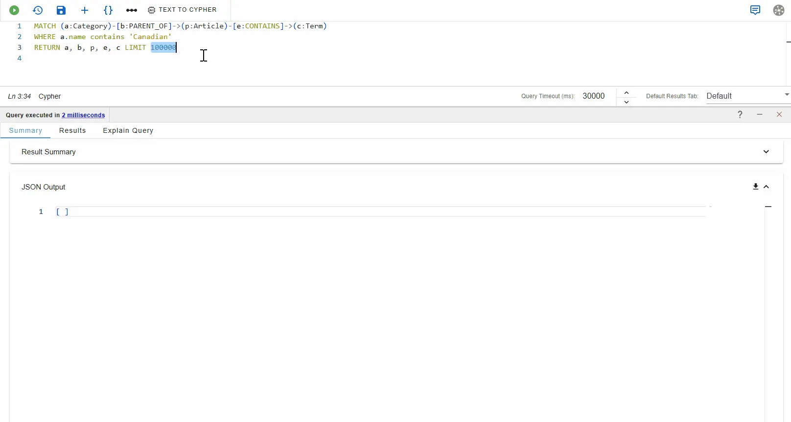
Figure 19: A more complex large query.
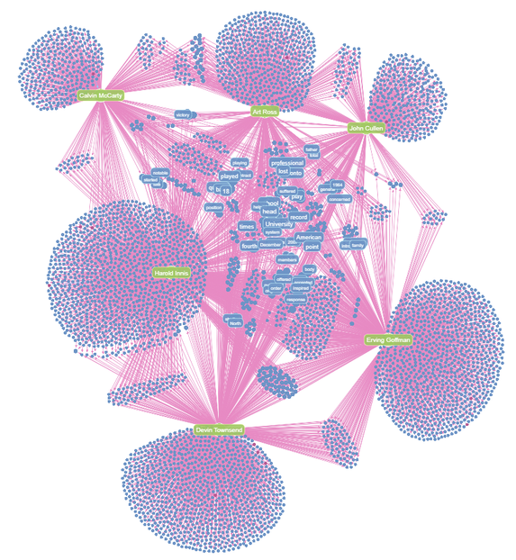
Figure 20: Here we’ve pulled out all the Article nodes (and the adjacent Term nodes) that contain the word ‘Canadian.’ Term nodes shared by a small number of Article nodes tend to cluster together – which might suggest that the two nodes have some similarity – for example Art Ross and John Cullen share many ice hockey Term nodes as both are ice hockey players.
Conclusion
Memgraph has a great developer experience – getting started with a sample dataset to explore takes just a couple of minutes, and Memgraph Lab offers all the essentials to get familiar with Memgraph. As you’re getting more familiar with graph data and start needing more advanced tooling to write queries and explore your graph, we’ve got your back.

![Cypher Labels: How to Organize Graph Nodes [Byte-Sized Cypher Series]](https://gdotv.com/wp-content/uploads/2026/01/labels-vs-properties-byte-sized-cypher-query-langauge-video-series.jpg "Cypher Labels: How to Organize Graph Nodes [Byte-Sized Cypher Series]")
![Announcing Ontology Support, Improved Data Model Visualization, Entra ID auth Support & More [v3.51.108 Release Notes]](https://gdotv.com/wp-content/uploads/2026/01/apache-age-entraid-auth-support-ontology-data-model-viz-gdotv-release.png "Announcing Ontology Support, Improved Data Model Visualization, Entra ID auth Support & More [v3.51.108 Release Notes]")