Getting started on Aerospike Graph with G.V() – Gremlin IDE

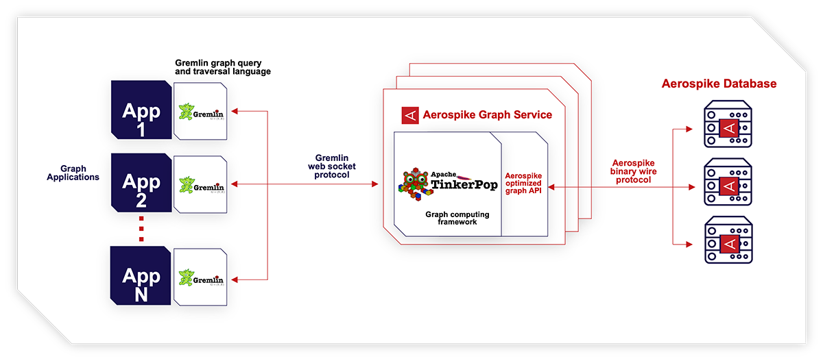
In this article, we’ll cover how to visualize and query your Aerospike Graph database using G.V() – Gremlin IDE. To support this, we’ll use a sample movies dataset that we’ll load on our Aerospike Graph database and discover interactively on G.V(). We’ll also write and explain some Gremlin queries to extract valuable information for the dataset via Aerospike Graph.

Before we start, let’s quickly introduce Aerospike Graph and G.V().

Aerospike Graph is a new massively scalable, high-performance graph database launched on June 23 2023 as part of Aerospike’s multi-model NoSQL database. It uses Gremlin as its main querying language and reports < 5ms latency for multihop queries, even for graphs comprising of billions of elements. It was also recently made available on the Google Cloud Marketplace.

G.V() is a Gremlin IDE – its purpose is to complement the Apache TinkerPop database ecosystem with software that is easy to use and install, and provides essential facilities to query, visualize, and model the graph data. If you want  to find out more about G.V(), check out From Gremlin Console to Gremlin IDE with G.V().

gdotv and Aerospike have partnered to offer a 60 days free trial of both Aerospike Graph and G.V() that you can take advantage of now if you haven’t already!

To  get started, you’ll need the following:

• Download Aerospike Graph: Have a running instance of Aerospike Graph as described in Aerospike’s Getting Started documentation with a folder of your choice mounted to the /etc/default-data folder of your container.
• Install G.V(): Download and install for free.
• A dataset: This movies dataset can help you get you get started. 

Once you’ve done all the above, you’ll be ready to connect G.V() to your database and visualize your data.

Connecting G.V() to your Aerospike Graph Database

Connecting G.V() to your Aerospike Graph database is quick and easy. 

If you’re running your Aerospike Graph database from a networked device, ensure  that the machine you’re running G.V() from can connect to the device. Refer to the demo below for  connecting to an Aerospike Graph database run locally on the same device as G.V():

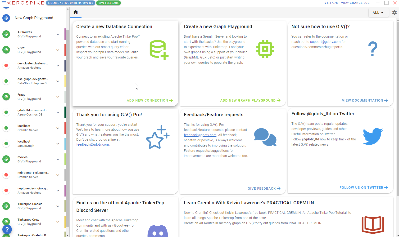
Follow these step-by-step instructions: 

• Click on New Database Connection.
• Enter the hostname of your Aerospike Graph database; if running on your local machine, this will just be localhost.
• Click on Test Connection. G.V() will make sure it can connect to your Aerospike Graph container. It will then present  a final screen summarizing your connection details, which you can now save by clicking Submit.

Once you’ve created the connection on G.V(), you’ll first be prompted to sign up for your 60 days free, no obligation trial of G.V(). Pop your details in there, enter your validation code, and you’re all set. 

This will transition to a new query window fetching the first 100 edges of your database, which should result in an empty array as we’ve not yet loaded data in our database.

Loading the Movies dataset in Aerospike Graph

Now that your Aerospike Graph database is up and running in G.V(), let’s load some data. Make sure you’ve mounted the volume to your Aerospike Graph Service Docker container, pointing either to a folder with the Movies dataset or to the dataset file itself.

For instance, in our setup, we’ve mounted our local default-data folder containing movies.xml to /etc/default-data. To load the movies.xml dataset in our database, let’s run the following query:

g.with("evaluationTimeout", 200000).io("/etc/default-data/movies.xml").read().iterate()

Give it a minute to run. Once complete, our dataset is loaded, and we’re ready to play with the data!

Styling the graph visualization

Let’s run a query to quickly visualize our data and get a good overview of the graph’s data model. In your G.V() query editor, run the following query:

g.E().limit(250)

Nothing fancy here – we’re just loading the first 250 edges in the database to generate a little display of your graph database. This is just to give you a taste of what G.V() can do!

Before we move on to our next steps, let’s quickly stylize the graph to make sure we’ve got the best display. To speed this along, we’ve created a stylesheet that you can import in G.V(). Download it here and follow the instructions below.

On the Graph view, click on Graph Styles as highlighted below:

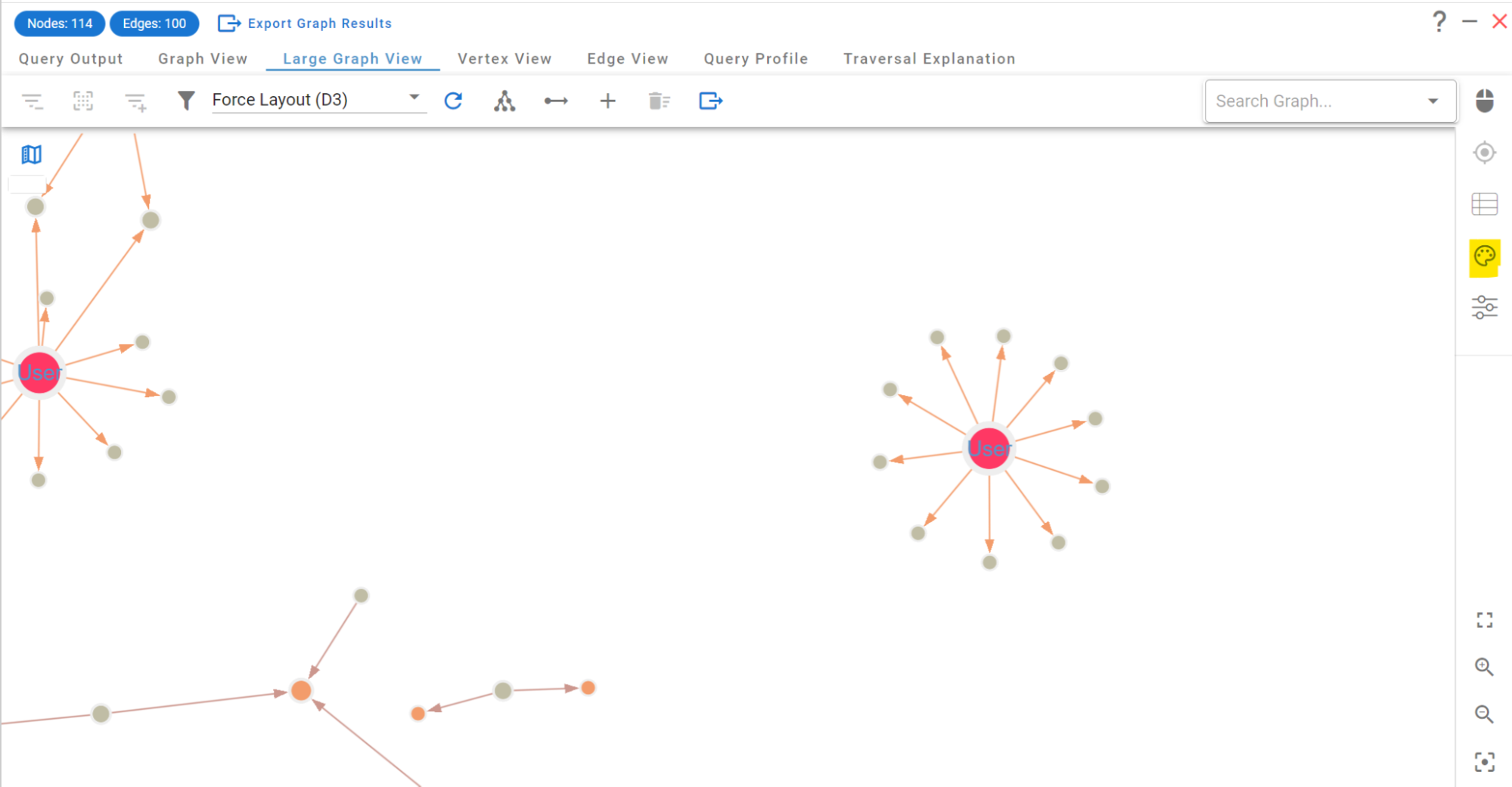
Next, click on “Import Stylesheet”:

This will open a file explorer in which you need to select the “movies-aerospike.json” file you’ve just downloaded.

Once loaded, click on “Save New Stylesheet.” After the stylesheet is saved, toggle it to be the default stylesheet by clicking on “Set As Default Stylesheet” – Done!

You’ll see that the graph now displays the relevant information directly on screen, as shown below:

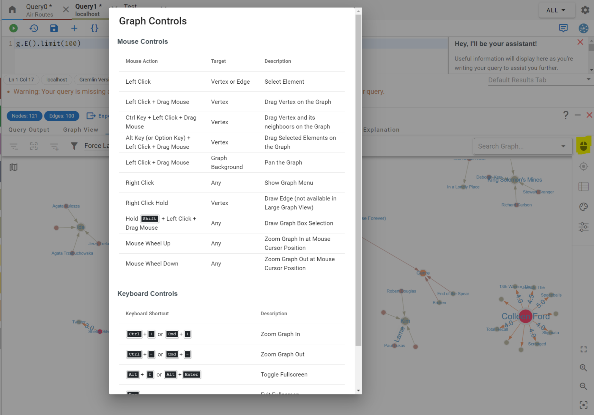
There are a lot of other things you can do in the graph view, so feel free to play around with the graph display. For reference, these are the graph controls and how to display them:

Exploring our graph’s data model

Once you’ve had a little interactive browse of your data, head over the Data Model Explorer view so you can examine the data structure:

As shown in the Data Model Explorer, our graph contains the following vertices:

• Movie
• Genre
• Actor
• Director
• ActorDirector
• User

Relationships in this graph are as follows:

• Movies are in a genre (IN_GENRE)
• Users have rated movies (RATED)
• Directors have directed movies (DIRECTED)
• Actors have acted in movies (ACTED_IN)
• ActorDirectors have acted and directed in movies (ACTED_IN and DIRECTED)

It’s all pretty self-explanatory (and that’s the beauty of graphs!). We’ll not enumerate all the properties here, but let’s just go over the main ones of relevance: 

• All vertices have a name property
• The RATED edge has a rating indicating the rating a user gave to a movie
• All vertices but Genre and User have a poster property containing an image URL and a URL property pointing to their IMDB page

Querying, analyzing and visualizing the graph

There’s a lot of useful information that we can leverage to query our graph and get some insights. Let’s give it a go:

Our first query is going to be simple. I just want to see the graph surrounding the Titanic movie:

g.V().has("Movie", "title", "Titanic").bothE()

Quick breakdown:

g.V().has(“Movie”, “title”, “Titanic”) finds any vertices with a Movie label and a title property that equals “Titanic” – makes sense so far.

The .bothE() bit at the end there says, “fetch all incoming and outgoing edges to the vertices”, in other words, it will fetch all relationships to the Titanic movie.

To run the query, first, enter it in the query editor as shown below, then click on the green play button. 

Quick note: If you click on the individual steps in the query, you’ll be able to see the official Gremlin documentation in the Gremlin Query Assistant on the right side of the editor. Great way to learn or remind yourself of the various steps and how they work:

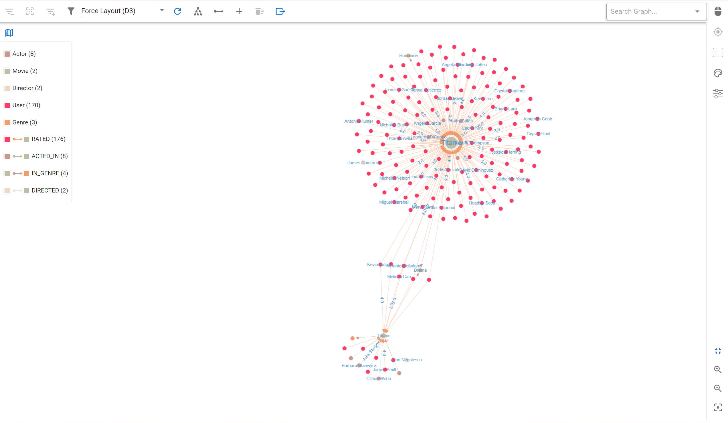
Anyway, once you’ve run the query, you’ll be presented with a graph display of the resulting data, and you should notice something odd: there are two Titanic movies! 

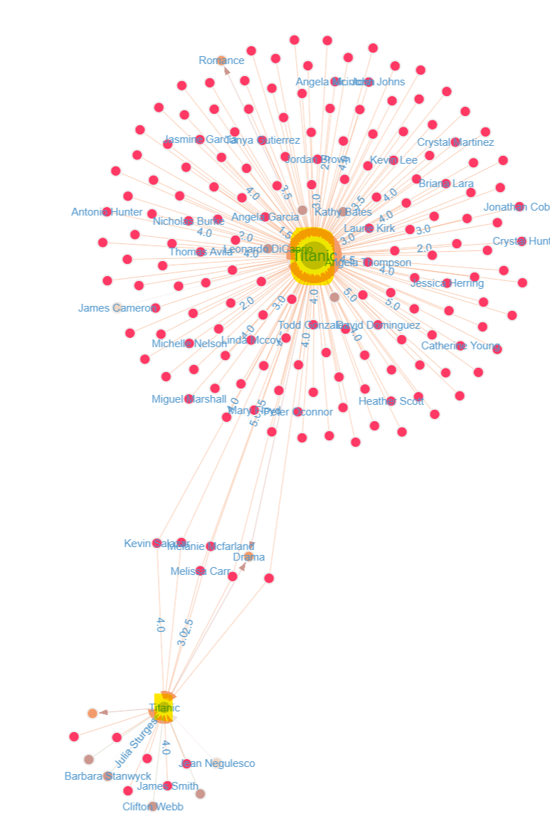
(Now of course there’s nothing odd here – there are indeed two Titanic movies but I for one was born in the 90s and I have missed the release night for the first one by just about 40 years)

The graph display also visually indicates that one of these Titanic movies has many more reviews than the other. Unsurprisingly, it is James Cameron’s version, as highlighted by the DIRECTED_BY relationship between Titanic and James Cameron.

Well, it’s simple: it just turned out James Cameron’s Titanic wasn’t the only one or even the first to come out! 

If you click on the Titanic nodes, you’ll also be able to check out their posters or open their IMDB movie page, as demonstrated below:

Let’s try a more complex query. What are the top 10 movies with the most user ratings?

g.V().
  hasLabel("Movie").
  order().by(inE("RATED").count(), desc). values("title")
  limit(10)

Here’s the breakdown of the query:

First of all, we’re only interested in movies, so  filter the  vertices accordingly with g.V().hasLabel(“Movie”).

Next, order these movies by a metric, in descending order, and get the first 10 results, which happens at:

order().by(…, desc)

Now, for the order itself, use the count of incoming RATED edges as the main metric , which is done via inE(“RATED”).count().

Finally, to display the title of the matched movies and limit this to a top 10, add values(“title”).limit(10)

The final result is (drum roll please):

==>Forrest Gump
==>Pulp Fiction
==>Shawshank Redemption, The
==>Silence of the Lambs, The
==>Star Wars: Episode IV - A New Hope
==>Jurassic Park
==>Matrix, The
==>Toy Story
==>Schindler's List
==>Terminator 2: Judgement Day

Now, these are all pretty good movies, but they’re not the highest rated films .

In this database, there are two types of ratings available:

• User ratings from 0 to 5 as shown in the RATED relationship from User to Movie
• IMDB ratings based on votes which are aggregated into the rating property of movies

Let’s start with the easy one: IMDB ratings.

g.V().hasLabel("Movie").order().by("imdbRating", desc).values("title").limit(10)

We get the following results:

==>Band of Brothers
==>Civil War, The
==>Shawshank Redemption, The
==>Cosmos
==>Godfather, The
==>Decalogue, The (Dekalog)
==>Frozen Planet
==>Pride and Prejudice
==>Godfather: Part II, The
==>Power of Nightmares, The: The Rise of the Politics of Fear

Okay, I don’t know half of these, but then again I’m no movie critic. Let’s change the query slightly to also include the rating of these movies:

g.V().
  hasLabel("Movie").
  order().by("imdbRating", desc).
  project("title", "imdbRating").by("title").by("imdbRating").
  limit(10)

This now results in the following:

==>{title=Band of Brothers, imdbRating=9.6}
==>{title=Civil War, The, imdbRating=9.5}
==>{title=Shawshank Redemption, The, imdbRating=9.3}
==>{title=Cosmos, imdbRating=9.3}
==>{title=Godfather, The, imdbRating=9.2}
==>{title=Decalogue, The (Dekalog), imdbRating=9.2}

==>{title=Frozen Planet, imdbRating=9.1}
==>{title=Pride and Prejudice, imdbRating=9.1}
==>{title=Godfather: Part II, The, imdbRating=9.0}
==>{title=Power of Nightmares, The: The Rise of the Politics of Fear, imdbRating=9.0}

Let’s enhance the query a bit further by including the director and actors in these movies.

g.V().
  hasLabel("Movie").
  order().by("imdbRating", desc).
  project("title", "imdbRating", “directedBy”, “actors”).by("title").by("imdbRating").by().by().
  limit(10)

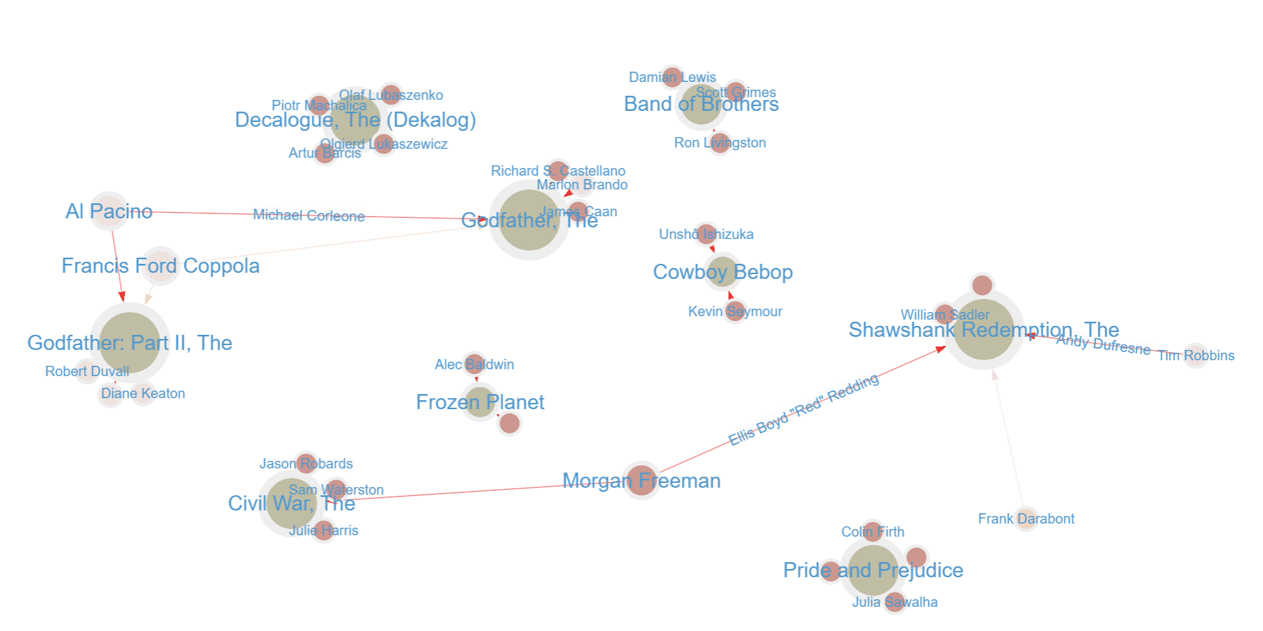
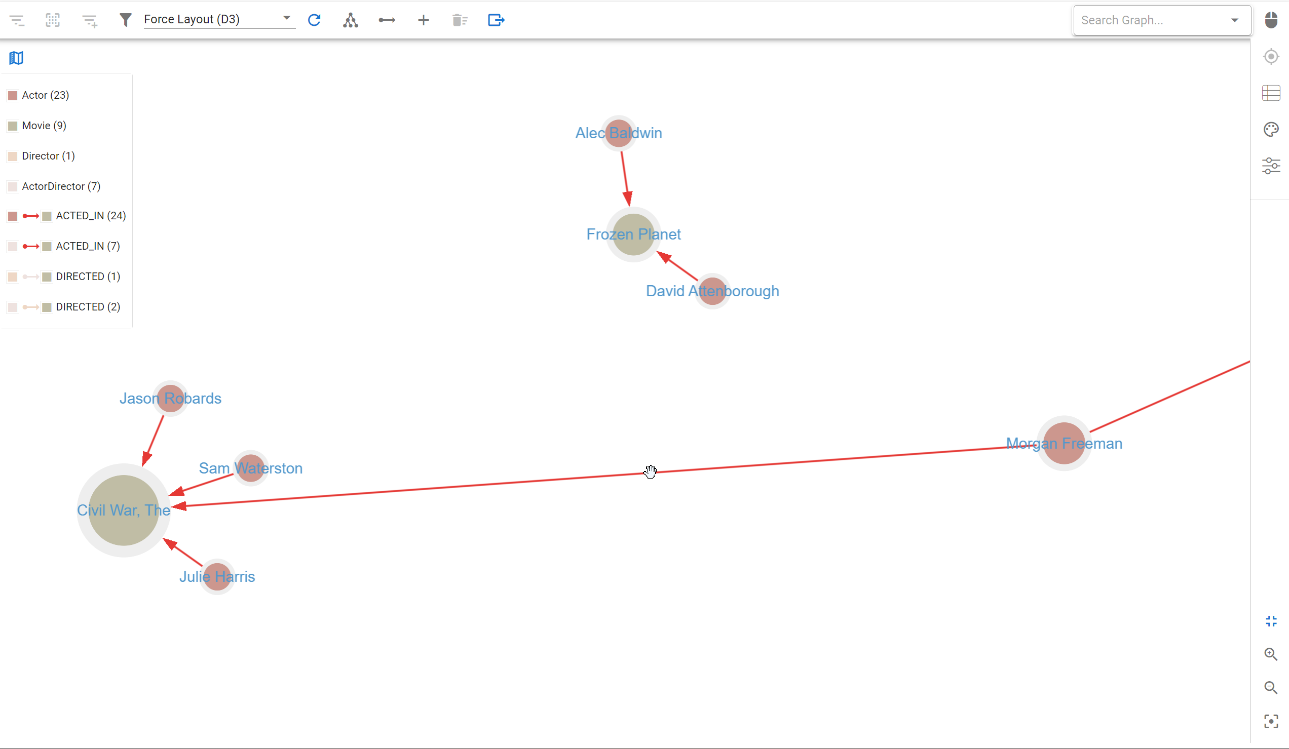
We get the following visualization:

At a glance, we can see that Morgan Freeman and Al Pacino both acted in two top-rated IMDB movies and that Francis Ford Coppola directed two of them, as well.  This kind of makes sense, given that for the latter, both movies are part of the same trilogy, The Godfather.

Just to wrap things up in this first introductory post, you’ll notice that some of the actor relationships are missing information; for instance, Morgan Freeman’s role in The Civil War is not stated. Using our graph visualization, we can easily update the graph interactively to fix any missing data. I will also add myself as an actor on Pride and Prejudice in this dataset, just because I can!

Try Aerospike Graph and G.V() free for 60 days

We’re just barely scratching the surface of what Aerospike Graph and G.V() can deliver together. This post simply demonstrates how you can quickly get up and running with a sample dataset on Aerospike Graph to explore graph data interactively or via Gremlin queries.

For instance, Aerospike Graph offers a Bulk Data Loader that can load your semi-structure CSV data into a graph database, enabling fast access to visual insights and interactive editing via G.V().

And as a reminder, here’s the best part: you can try this all out for 60 days for free! So what are you waiting for? Get your Aerospike Graph 60-day trial now and explore your shiny new graph database with G.V()!