Game changer? A first look at the Hydra project

Introduction
Part 1: Introducing Hydra
What’s Hydra?
Hydra is a programming language that uses mathematical abstraction to model graphs within the language itself. It’s an open-source project spearheaded by Josh Shinavier, co-creator of Apache TinkerPop. In Josh’s own words: “In Hydra, programs are graphs, and graphs are programs.”
Though the technical side might get a little gritty – the end result is elegant and powerful: Hydra empowers users with a toolkit of functions and DSLs (Domain Specific Languages) to transform and validate graph data and schemas with maximum versatility across types and standards.
Hydra’s strength lies in breaking graphs down into their fundamental components, passing all schemas and data through its own core data model. Using these building blocks, Hydra exploits compositionality to allow definitions of arbitrarily complex and interlocking
data transformations. So you can not only build and translate graphs, but entirely re-compose your data from scratch. This approach allows extremely dynamic schema within a framework of robustly consistent logic, and helps to navigate tricky areas, like heterogeneous environments and interactions with relational and other non-graph data.
The language will have full parity across multi-language implementations, with a Haskell implementation already complete and Python and Java forms in progress.
In this post we’ll use Hydra for a simple and familiar use case – transforming relational data into graph form. This will serve as an introduction to some basic Hydra DSL, yes, but more importantly, it will give you a glimpse of just what’s possible within Hydra. The flexibility Hydra offers within our simple example is just a taste of what the final project will be capable of.
Use Hydra locally
Hydra is currently accessible from its GitHub repository . Since development is still underway, the easiest way to get started is via the /hydra-ext subproject which has been created specifically for demo use. Our demonstration today is an adapted version of the GenPG demo in /hydra-ext using some of our own data and code that we’ve linked for download.
Note that this demo uses the Haskell Hydra implementation and following along yourself will require installation of the Haskell Tool Stack. We’re not going to linger too long on the intricacies of Haskell itself, but A Gentle Introduction to Haskell will give you the fundamentals. We’ve also provided all the code used in this tutorial along with the corresponding outputs, so you’re free to follow the guide and examine all the components individually without needing to run anything yourself.
Part 2: Unleashing Hydra
Example scenario
Let’s imagine we work for a vet’s office that’s been storing all its data in simple spreadsheets.
We have records of the various pets and their owners recorded in the pets.csv and owners.csv files. Many of these owners have appointments next week concerning their pets, and the information for this is stored in appointments.csv.
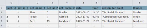
Some of the pets get on better than others, so a member of staff thought it would be useful to document animals that get on particularly well. This is stored in the pet_friendships.csv, while incidents between animals are recorded in pet_fights.csv
Someone pointed out that if we want to schedule a new appointment for a pet, it would be useful to see all this data laid out in a graph format.
Start out by downloading our sample dataset here:
vet_office
This includes five relational .csv files:
| File name | Preview |
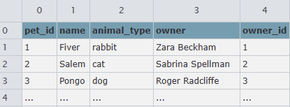
| pets.csv |
|
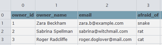
| owners.csv |
|
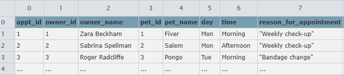
| appointments.csv |
|
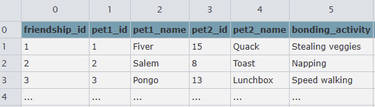
| pet_friendships.csv |
|
| pet_fights.csv |
|
Planning your strategy
We have relational data. We’d like to have graph data instead.
This is where Hydra comes in. Hydra DSL equips you to dynamically construct a graph transformation on the basis of virtually any input. To start with a simple example, let’s devise a schema for what we’d like our final product to look like:
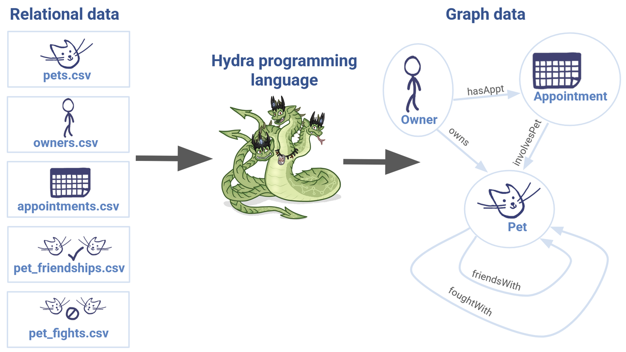
The transformation that we’d like to make from relational data to graph data.
As we can see, three of our .csv files map to vertices – Owner, Appointment and Pet – and two of them map to edges – friendsWith, foughtWith. (Note that we’ve deliberately kept it simple for now! We’ll explore something a little more ambitious later on.)
In order to transform our data, Hydra needs to know three things:
- The structure of the input data (a relational database in our example)
- The structure of the output database (a graph database in our example)
- How the input and output databases relate to each other
For ease of readability, we’ll spit these components into three separate files:
DatabaseSchema.hsGraphSchema.hsMapping.hs
Where the .hs extension simply designates that these are Haskell files.
So our transformation now looks like this:
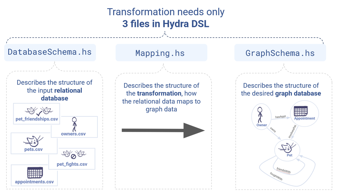
The three Hydra files that will form the basis of our transformation.
Implementing your idea
Now that we understand what we want to do, we need to actually start writing Hydra code.
Getting started here might take a little time. Currently, there are no simple tutorials to learn Hydra DSL itself. If learning seems daunting, one option is that you can use a LLM (like Claude) to write your Haskell files for you. This is what is suggested in the demo – there is even an included python script to generate a custom prompt.
Of course, whether you choose AI assistance or not, understanding any programming language always provides the greatest measure of control and validation when using it. That’s why we’ve provided you with a few example files to get familiar with Hydra DSL.
Download them here:
hydra_v1
This .zip file contains our three Haskell scripts, pre-written to correspond to the vet office data you already downloaded: DatabaseSchema.hs, Mapping.hs and GraphSchema.hs. Each one is written in a Hydra DSL.
Let’s start with DatabaseSchema.hs. Remember, this is where we define our input (relational) data. Since our input is just five .csv files, we define five functions with the following basic format:
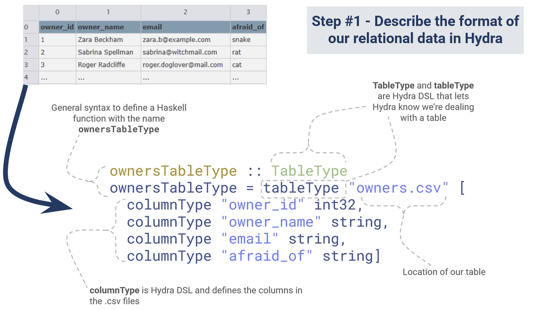
A description of our relational data.
Each function is defined as an instance of tableType in Hydra DSL, with the columns extracted using the columnType Hydra DSL. This defines how to read each .csv, including what kind of data we expect to see in each column (as an aside: static typing is a very important part of both Haskell and Hydra’s strengths! It’s so important that it’s even maintained across other implementations via the use of phantom types). Already we are getting a hint of the versatility of Hydra – the input data doesn’t have to be in a simple table format like this – there’s the potential to get far more adventurous with our inputs.
Now let’s look at the structure of our target output data, as defined in GraphSchema.hs. Similarly to before, we define three vertices and three edges with the properties we want:
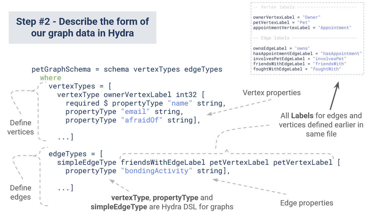
A description of our graph data.
We’ve defined a schema using the vertexType, edgeType and propertyType functions, which are part of Hydra’s property graph DSL. Note that we haven’t yet populated the graph with any of our data! This is just an abstract representation of the data model.
The last step is to define the transformation, this happens in the Mapping.hs file. This is likely the trickiest file to understand without Haskell or Hydra knowledge. But you should hopefully be able to see that the Mapping.hs file maps out how to populate the graph using data from the .csv files.
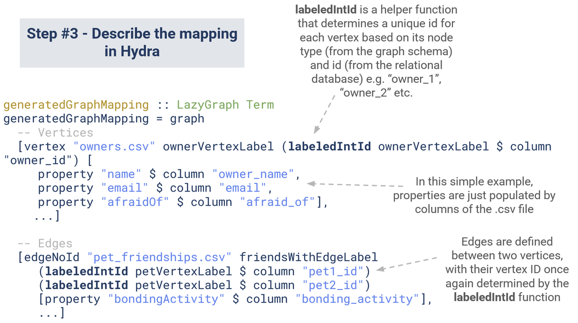
A description of the mapping between our relational data and our graph data.
(If this seems similar to the previous DatabaseSchema.hs file, then that’s reasonable. DatabaseSchema.hs showed how to read the input tables, Mapping.hs says what to do with the tables.)
Transforming with Hydra
With these three scripts, we’re ready to make our graph! To do this, we use one of Hydra’s built-in transformations.
The demo we mentioned previously provides a sample function generateGraphSON which will do this for you. It’s located within the Demo.hs script located at: hydra/hydra-ext/src/main/haskell/Hydra/Ext/Demos/GenPG
If you make sure your new scripts are imported correctly and the data is located in the right place (consult the demo for more information) you can build your Haskell stack and run the following command:
generateGraphSON "data/genpg/sources/vet_office" generatedTableSchemas generatedGraphMapping "data/genpg/vet_office.json"
This results in a standard GraphSON file (a kind of .json file, detailed here), which we can effortlessly explore in G.V().
For your convenience, you can also download the output file here:
vet_office_v1.json
Adding G.V() to the equation
If you don’t already have G.V(), head on over to the download portal. Once you have it installed, it will only take a few seconds to import your new graph.
Just click on New Graph Playground. You’ll have the option to Import your own data in GraphSON format, and just like that, you’ll be able to instantly visualize your new dataset.
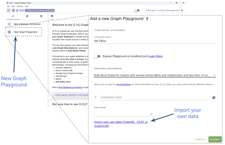
Create a new playground in G.V().
Exploring our result in G.V()
We can get an overall view of the graph structure by viewing the Data Model, and we can see right away that this corresponds to the schema we sketched out previously.
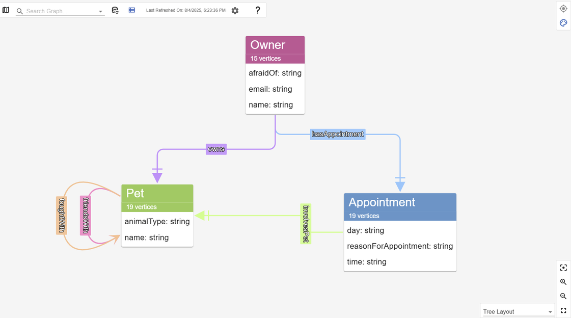
You can view the data model within G.V().
A straightforward g.E() command gives an overall view of all the nodes and edges in the graph that Hydra has constructed:
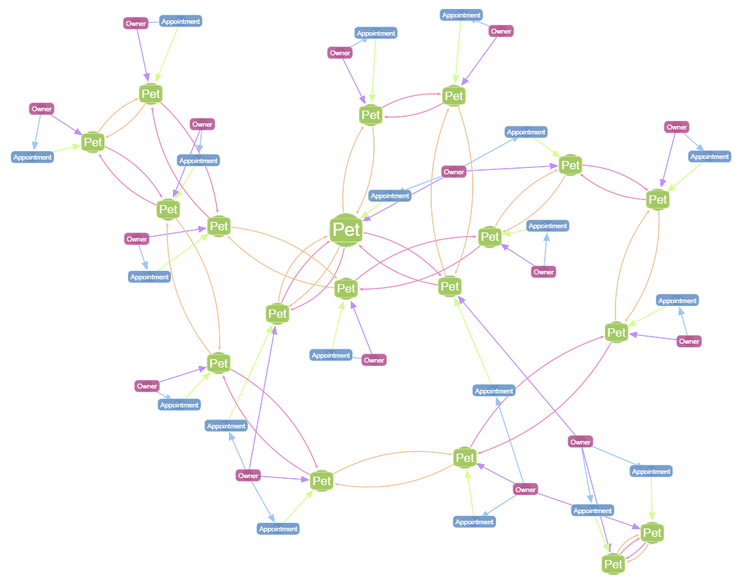
An overview of our new graph data shows that the relationships from our .csv files have been well-preserved!
To illustrate the advantage of our new graph model, let’s say we wanted to schedule pet appointments with some simple rules. For example, if two animals are friends, we’d like to try and book them in at the same time. (But we want to avoid concurrent appointments for pets that have fought together in the past!) We can run a straightforward query, or use the Graph Data Explorer to explore relationships between pets at a glance:
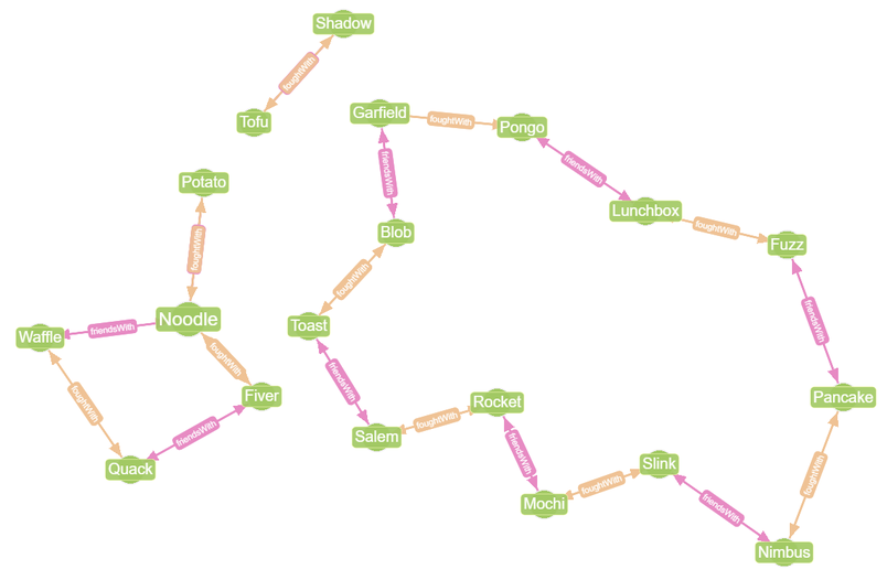
An example use case of this data could be to see relationships between the various pets.
Part 3: Iterating with Hydra
Evolving our schema
What if we wanted to create a new node from columns in our .csv files? For example, every pet in the pet.csv has an associated animal_type property that lists the species of the pet, such as cat, dog, rabbit etc. Similarly, the owners.csv also lists animals the owner has a particular fear of in the afraid_of column.
Right now, Hydra just interprets each row in the .csv as a vertex, and these columns are just assigned as properties of the Pet and Owner vertices. But what if we wanted to do something different? What if we wanted to associate each unique animal in the pets.csv as its own vertex?
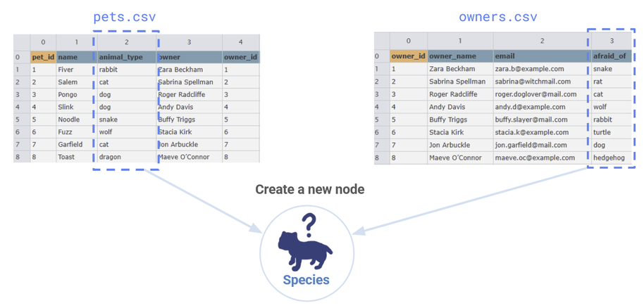
We see that we have the information to create a new node from the species columns of our .csv files.
Furthermore, what if we wanted to attach new edges to this vertex, letting us know which pets correspond to that species, and which owners are afraid of that species?
Our new data model would look like this:
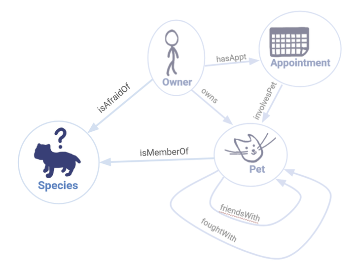
Our updated data model incorporates the new node that we have created.
We’ve prepared a new set of Hydra files that will show you how to do just that:
Download them here:
hydra_v2
The major changes are two the Mapping.hs file, where we have defined our new edges and vertices:
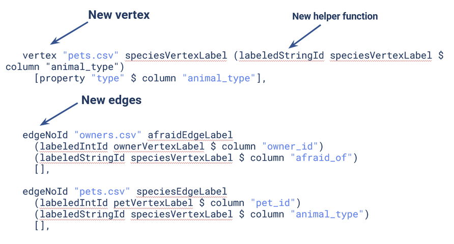
Our updated Mapping.hs file now informs Hydra that we want to create a new node with new associated edges.
This new vertex is also constructed using data from the pets.csv file. Note the inclusion of a new helper function labeledStringId.
What’s the purpose of this new function? Well, the previous nodes were all defined by a unique integer ID column in the .csv file itself. For example, Zara Beckham has the owner_id entry with value 1, so her node is assigned the label owner_1. Sabrina Spellman becomes owner_2, etc.
However, our new species node has no such unique identifier by default, so we have to construct a new label. We’ve chosen to assign each node a unique label using each unique string in the animal_type column, e.g. species_cat,species_dog. Because our new function deals with a string instead of an int, we redefine a new version of the function to deal with strings. This may seem redundant, but the static typing of Haskell is among its strengths!
Once again, you can run the code yourself or simply download the output from here:
vet_office_v2.json
Review with G.V()
View the updated Data Model:
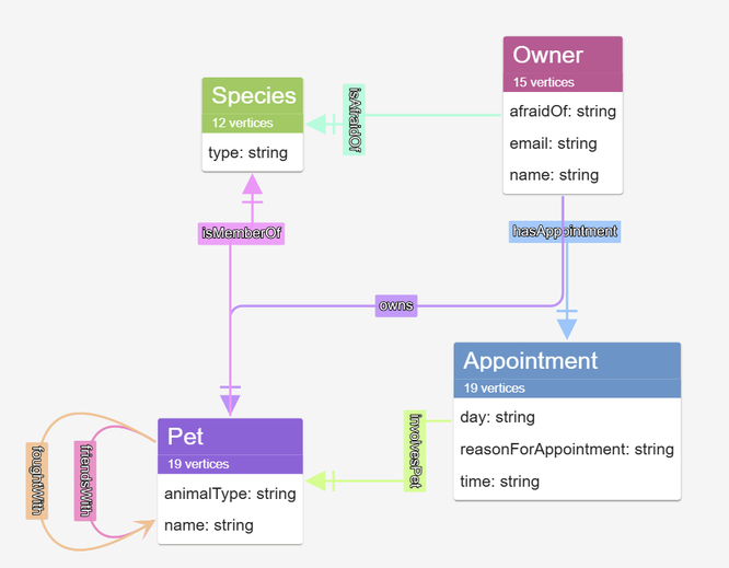
Our updated data model reflects the inclusion of the new node.
Can view the relations around e.g. the cat node, showing which pets are cats and that you might want to keep Roger Radcliffe out of the office when any of them are around!
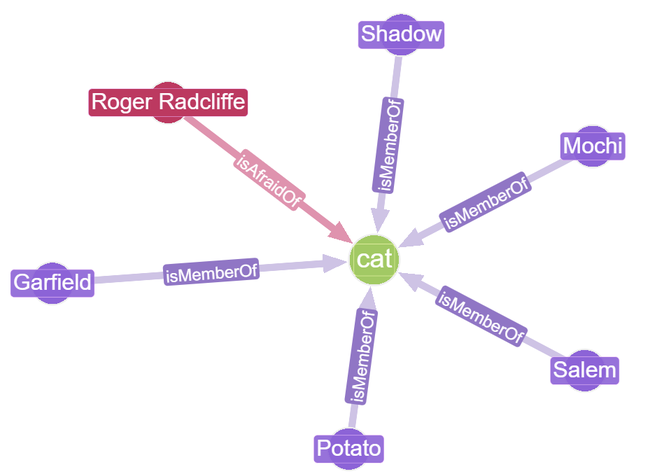
This ‘cat’ node is an example of our new species node, displaying the new edge relationships we have assigned to it.
Conclusion & further reading
We’ve explored some first steps you can take with Hydra, but we’ve only scratched the surface of what’s possible with the broader machinery. While this early form of Hydra is not trivial to use, we hope you’ve caught a glimpse of what’s possible. Josh and the rest of the team are working tirelessly to bring the project to maturity, and future Python and Java forms will let you interface in your programming language of choice. The first step is to bring Hydra to the Apache Incubator path, hopefully in the near future, then introduce Hydra into the wider community.
Make sure to listen out for future updates. Links of further interest:
- The Hydra GitHub page – Where you can download the current version of Hydra
- The LambdaGraph data model – This is the foundation of Hydra. A mathematical model that illustrates how programs which operate on graphs are graphs themselves.
- The Hydra code-free demo – The demo that this demonstration is adapted from. If you found it tricky to follow our implementation, try this demo first!
- The original Hydra design document – A broad overview of the current and intended structure and features of Hydra.
- Join the LambdaGraph Discord – Get directly involved with the development community right away.


