From raw data to a knowledge graph with SynaLinks

Introduction

Here at G.V() we’re always on the look out for new graph technologies. That’s why we’re excited to introduce you to SynaLinks! SynaLinks is an open-source framework designed to make it easier to partner language models (LMs) with your graph technologies. Since most companies are not in a position to train their own language models from scratch, SynaLinks empowers you to adapt existing LMs on the market to specialized tasks.

SynaLinks is a Pythonic framework adapted from Keras 3, and built on a principle of progressive complexity. This allows you to customize your workflow to be as intricate as you want it to be. That means whatever your background, and even if you’ve never worked with an AI backend before, SynaLinks might have something to offer you. For newcomers, this could be a great opportunity to build your first interface. Conversely, if you’re an experienced developer, there’s a great deal of functionality within SynaLinks to explore.

Today, we’re going to give a brief overview of program construction in SynaLinks. One application that’s straightforward to implement is building knowledge graphs and running GraphRAG – so we’ll give a brief walkthrough of the former, and then direct you to where you can continue on with the latter, if you’re so inclined. We’ll use SynaLink’s own knowledge graph introduction, and then we’ll use G.V() to explore the results.

Getting started with SynaLinks

To install synalinks, you can use the following commands in your terminal of choice:

uv venv
uv pip install synalinks

You can then use the command uv run synalinks init  to initialize a sample project, if you like. If you do, you’ll be greeted with the initialization screen:

Figure 1: The SynaLinks welcome screen in the terminal.

From here you can customize some key features of your environment. We won’t focus too much on the details of the sample project here, but the first important decision for you is choosing a language model to connect to SynaLinks.

Note that you’ll need to have your own account with an associated API key to access a remotely hosted model. If you don’t have credentials with any such model provider, you can download Ollama to run a language model on your device for free, such as  ollama/mistral or ollama/deepseek-r1, on your local machine. You should be aware of the limitations of these small models, but they’ll function fine for proof-of-concept. That’s what we’ve used for this demonstration.

Note that you’ll also need to have a graph or knowledge base somewhere that SynaLinks can connect to. If you don’t have one already, the easiest way to do this is to host a Neo4j instance locally on your device via Neo4j Desktop.

Lastly, you’ll need to choose an embedding model, such as all-minilm or snowflake-arctic-embed – this will be used to embed your graph in a vector space, which SynaLinks will use to process your data more efficiently.

Example problem – building a knowledge graph

We’ll follow the knowledge graph example provided by SynaLinks, which starts from some basic .txt files with some  general information about countries in western Europe. Note that these are given in plain English. They contain information that could be used to construct a graph, but is not currently in graph form. For example, one file (modern_political_events.txt) looks like this:

The European Union summit took place in Paris in 2023, with leaders gathering to discuss climate policy. Paris is the capital of France and frequently hosts international diplomatic meetings. Brexit negotiations took place in London over several years, fundamentally changing the relationship between the United Kingdom and Europe. London is the capital of the United Kingdom and served as the center for these historic discussions.The Vatican Summit took place in Rome, addressing global humanitarian issues. Rome is the capital of Italy and often serves as a venue for international religious gatherings.

The general gist of the project is simple. Given this set of text, ask the Language model to produce a graph from the given data that encapsulates entities and relationships such as countries, cities, events and places, and their relationships to one another.

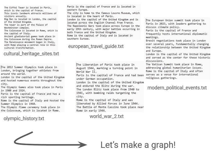
Figure 2: Example plain text files with some natural language information on western Europe.

We could represent our target graph with the following schema:

Figure 3: The schema for the target graph we’d like to make from our example .txt files.

Before we worry too much about how we’ll actually build the graph, the first step is to define some schema for what we want it to look like.

We can use the synalinks.Entity data model to define our nodes.

Here is an example of a defined City node:

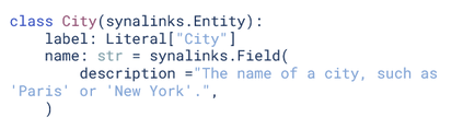
Figure 4: SynaLinks syntax to specify a node or ‘Entity’ in our schema.

Based on this model, we can create schema as above for the following four nodes:

• City
• Country
• Place
• Event

We can similarly use the synalinks.Relation data model to create a relationship:

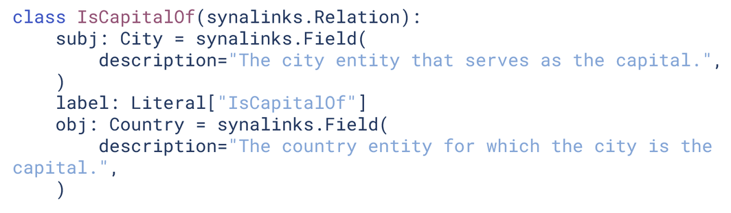
Figure 5: SynaLinks syntax to specify an edge or ‘Relation’ in our schema.

We create four edges this way:

• IsCapitalOf
• IsCityOf
• IsLocatedIn
• TookPlaceIn

Now that we have our schema nailed down, we’re ready to define our Program!

What is a Program?

The central element of SynaLinks is the Program. There are a number of ways to build a Program in SynaLinks, but we’ll focus on just one – functional style.

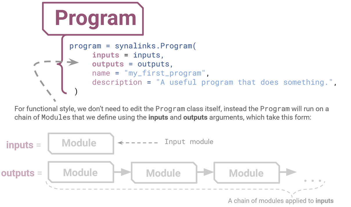
Figure 6: The basic structure of a SynaLinks Program. It consists of a series of modules, which are chained together and defined by two arguments; the inputs and outputs.

The easiest way to control the structure of the Program is via just two arguments – your inputs and outputs. This is functional style because we’re feeding our Program all the things you want to happen inside as a series of functions. The basic building blocks you use to define your inputs and outputs like this are known as Modules.

One way to picture a Program is as a kind of graph, made up of Modules as its nodes, which pass JSON data between them as edges. It’s a directed acyclic graph, meaning that information might branch out, but always flows in one direction. This could take a simple form like this:

Figure 7: A SynaLinks Program can be a simple chain of modules.

Alternatively, a program could have a more intricate layout like this one:

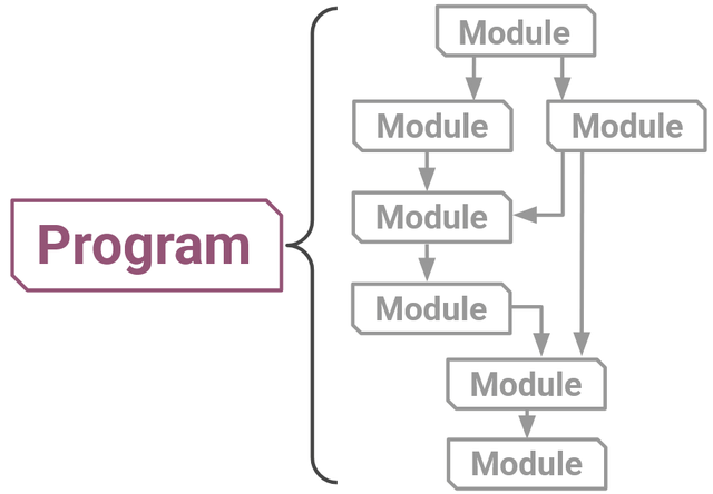
Figure 8: A Program can also consist of modules with a more complex, branching structure.

More discussion of how branching paths work can be found in the control flow section of the SynaLinks documentation. Note that a Program itself is a kind of Module, which can therefore be stacked or encapsulated in a larger Program!

Now that we understand the essence of what a Program is, we’re ready to dive into actually writing.

Writing our Program

You can see various examples of SynaLinks scripts for knowledge graph extraction in this folder on GitHub. Our approach closely follows the discussion on the Knowledge Extraction section of the SynaLinks documentation, which also uses the examples.

We’ll start with the simplest of these examples. which is a demonstration of one stage extraction, and is based on the script here.

By “one stage,” we mean that we’ll only have one type of conversation with our language model. Think of it like asking just one question – we might provide our language model with multiple datasets, but we’re going to ask it to do the same thing every time. (We’ll see later that we can have smaller, compartmentalized conversations with our language model – or even with more than one language model – if we want to exercise greater control over the individual elements of the workflow.)

In this example, we use four primary Modules to construct our Program. These are the Input module, Generator module, Embedding module and the UpdateKnowledge module.

In order, these Modules perform the following tasks:

• Input Module: This gives our Program information about what kind of input to expect, which allows the program to process its input data. For example, we are expecting text files, so we can use this module to set the data_model to Document.
• Generator Module: This is the part of the program that will interact with the language model. This takes our input data model (such as our input .txt files) along with a target data model (our target schema that we defined before) and consults with the language model to produce an output.
• Embedding Module: This creates a vector embedding of the data, i.e. takes the high-dimensional output of the previous step and converts it into a low-dimensional space. If you’re not familiar with vector embedding, all you need to know is that this step is necessary so that SynaLinks can process the data efficiently.
• UpdateKnowledge Module: Uses an embedded knowledge graph to update an existing knowledge graph, which could (for example) be your locally hosted Neo4j instance.

The overall program then has this general form:

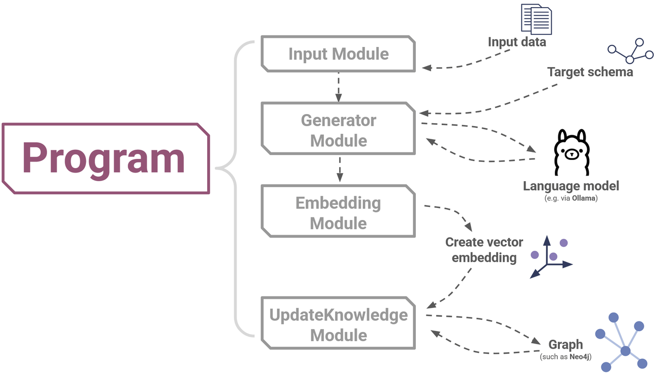
Figure 9: The basic structure of a simple, one-stage knowledge construction pipeline in SynaLinks.

Make sure to take a look at the code, and see if you can identify where each step is happening. It’s actually more intuitive than it may seem at first!

Examining the output with G.V()

G.V() is a great way to view your final output graphs, perform some quality control and analyze the resulting graph data.

In fact, if you really want to get a feel for how SynaLinks works, you can even get a real-time view of your data as it’s being generated!

If you don’t already have G.V() installed, it’s as simple as heading over to the free download portal to grab your free trial. Then you can open a New Database Connection.

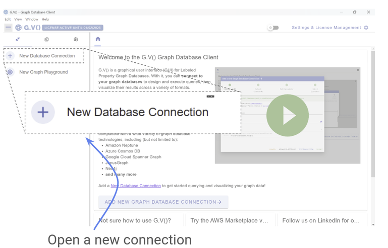
Figure 10: Connect to your graph with G.V().

From there it’s only a few clicks to connect to your graph (if you’re running Neo4j locally, simply use localhost as the hostname) :

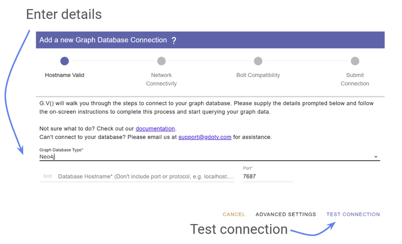
Figure 11: Input your graph details to connect.

SynaLinks even have their own tutorial on using G.V()! So check that out, open up G.V(), and get connected and comfortable.

Once you’ve opened your graph with G.V(), you can watch the output as it is generated:

Figure 12: The SynaLinks graph is generated iteratively, which you can see in G.V().

This is a great way to understand how SynaLinks procedurally pieces together your graph.

CAVEAT – “Why are some of the results wrong?”:  It’s well-known by now that language models are known to have difficulty discerning truth and therefore have a tendency to produce plausible but incorrect statements known as hallucinations. We want to stress that the quality of inference is a function of the language model used, not SynaLinks itself.

What’s going on behind the scenes?

Part of the advantage of SynaLinks is that you don’t really have to worry about what’s going on in the backend. But it’s still helpful to understand what’s happening in general terms so that you can optimize your workflow, so let’s take a closer look at the Generator Module.

Recall that the Generator is the part of SynaLinks that communicates with the language model. It takes your input data and target schema to prodata an output.

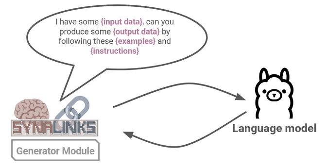
Figure 13: SynaLinks interfaces with the language model via a natural language prompt.

As you might expect, SynaLinks is prompting the connected LM with a classic text based prompt. This is the same as how you would communicate with an LLM chatbot, except that SynaLinks automates this process, integrating LM reasoning abilities to interpret your data, while ensuring the inputs and outputs conform to fixed regimented schema. The default prompt is stored in a jinja format and cleverly customized to fit your data by SynaLink’s own internal mechanics.

One important stability feature to mention is that the Generator module uses constrained decoding to make sure that the output completely respects the JSON schema. That means that, though language models may hallucinate some information within the graph, the overall syntax and schema of the graph is entirely preserved. The scope of possible error is then well-constrained by SynaLinks, and the overall structure of the graph cannot be broken, not even by mistakes caused by faulty LM inference.

By utilizing this Generator module in a clever way, we’ll see in the next section that we can customize and duplicate this component to greatly enhance the power of our Program.

Working with your language model

SynaLinks’ ability to generate the best knowledge graph possible is very dependent on the language model you use. In the example above, we essentially asked the language model to look at our input data and produce an entire graph at once, processing the full schema and all nodes and relationships.

A complex language model with a large context window and sophisticated reasoning abilities will be able to perform this task well, however a smaller model (particularly one hosted on your local machine) may struggle to complete the task to a high standard.

One way you can utilize control flow to help with this problem is to break large projects into smaller chunks. These chunks are easier for the language model to process and can be folded back into the pipeline once they are processed. Each of these chunks can be further modified and adjusted to make sure they perform as well as possible. This allows for greater control, more space for optimization, and increased versatility in your work flow.

For example, you could handle entity extraction and relationship inference by two separate language model conversations that are optimized for each task. Each conversation could happen with the same language model, or separate ones:

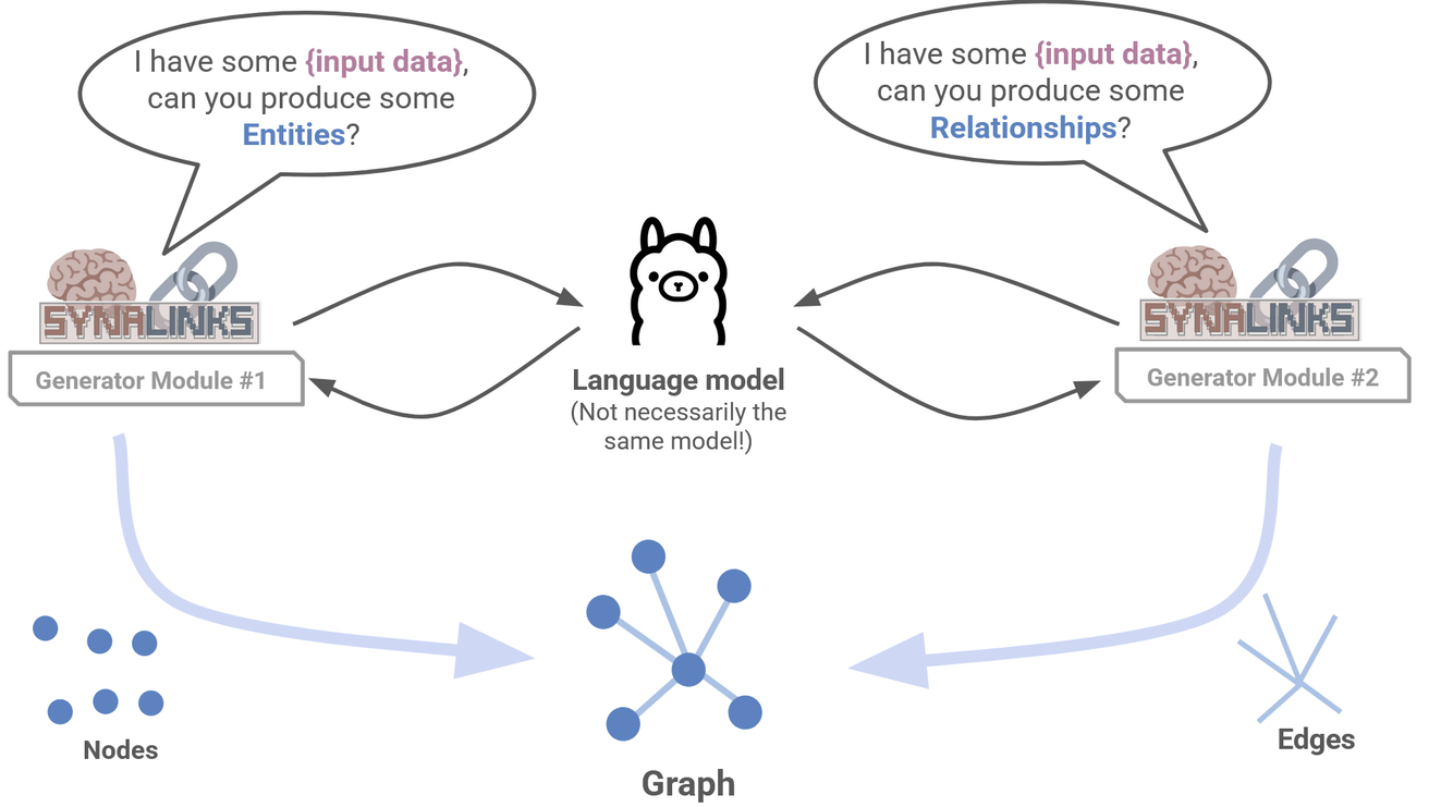
Figure 14: You can use multiple Generator modules to have multiple conversations with the language model.

The above is an example of two-stage extraction, and you can see an example of this given here.

But that’s just the beginning. You can extend this idea much further – to an arbitrary degree of complexity depending on your task and tools. As another example, you could have each entity and and each relationship all handled separately in the workflow. For our knowledge graph example, this would be a multi-stage extraction featuring eight different Generator modules handling four nodes and four relationships respectively.

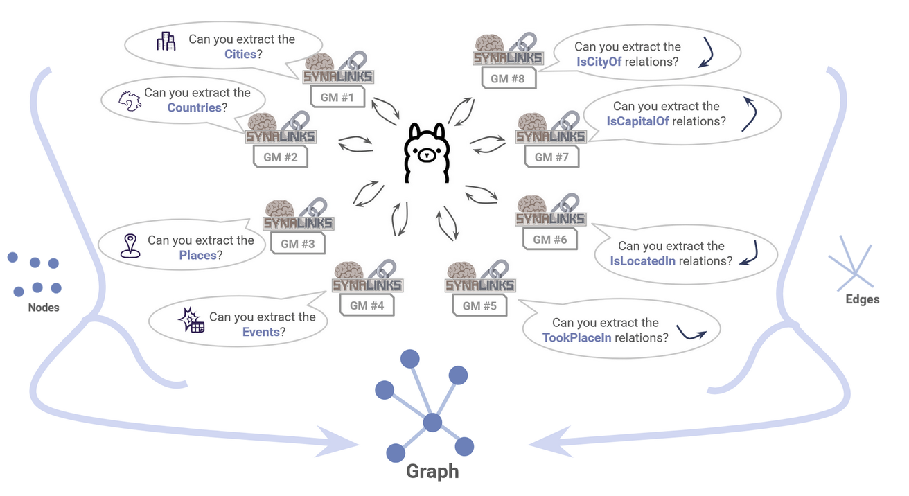
Figure 15: An arbitrary number of Generator modules can be used to exert greater control over each element of your workflow.

To see what that would look like, see this example.

Finding the balance between simplicity, efficiency and accuracy depends on both the project and the language model in question. The great thing about SynaLinks is that the modular format allows you amazing flexibility in the kind of workflow you can design.

As you can see, combining modules together can quickly create complex workflows that are powerful, but tricky to keep track of by hand. So, as a final point, we note that a great way for you to see the format of your Program is to use the plot_program() function, which automatically produces a .png image of your work flow!

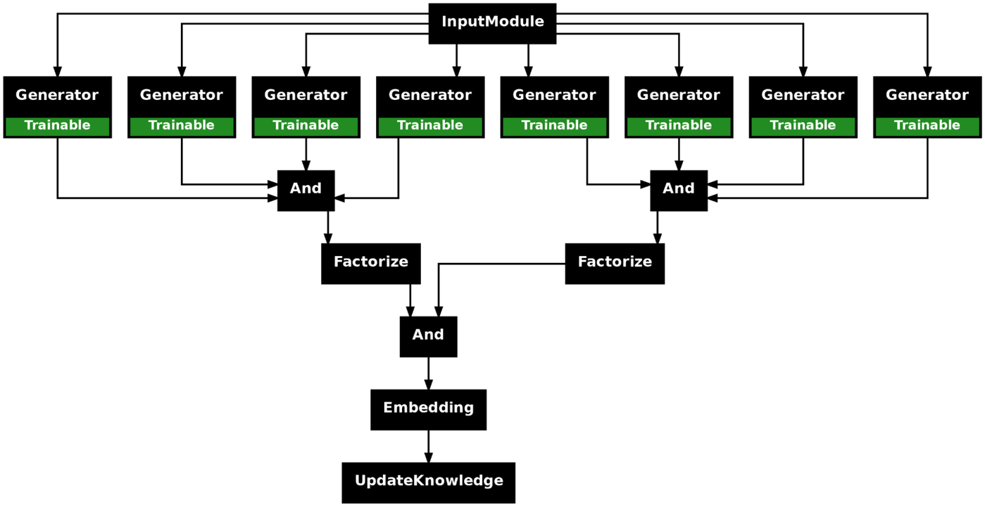
Figure 16: SynaLinks Programs can generate a .png file displaying their own structure. This is useful to understand how your pipeline is set up.

Continuing with retrieval-augmented generation

What about using your graph once you’ve built it? If you’d like to take the next step, SynaLinks encourages you to move forward into RAG applications, which are also supported by the framework.

We haven’t gone into that in too much detail, but the principle is the same. The Generator module will once again play a key role, and the new EntityRetriever module will be introduced. If you’d like to continue down this path, check out the next part of the SynaLinks knowledge graph tutorial.

Conclusion

We’ve reviewed just a small example of what anyone interested in graph technologies can achieve with SynaLinks, an exciting new tool for building and managing your projects. By building up your workflow piece by piece, SynaLinks lets you automate and integrate language model querying into your graph applications.

We’ve shown how that can be used to construct a graph, and we encourage you to push forward and see how SynaLinks can also be used for GraphRAG. Happy coding, and don’t forget to use G.V() to evaluate your results!