LadybugDB and Snowflake: Building a Graph From a Relational Data Store
‘Graph-on-relational’ is a hot topic these days.
It’s speculated that graph database technologies may be able to increase the speed and reliability of large language models in a way that could solve the technical deficit. With that in mind, people are looking for routes to leverage this combination in a way that could be profitable. Rather than building new graph-native databases, the idea is to build infrastructure on top of the established, ordered relational databases that already exist.
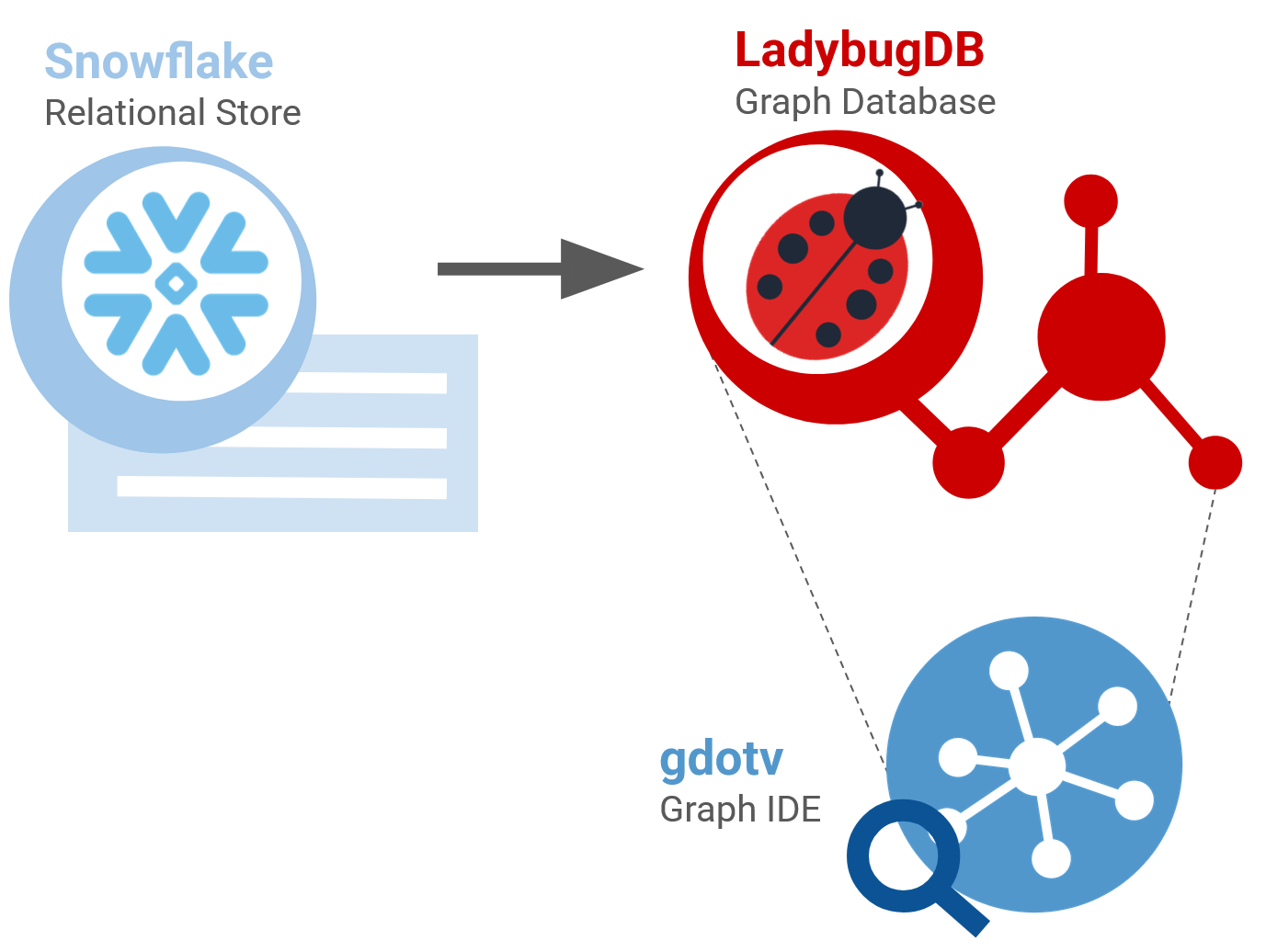
One difficulty is that relational data stores can be extremely large, which can make them unwieldy. Today, we’re going to walk through a particularly interesting example: we’re going to use new functionality implemented by LadybugDB to process a very large Snowflake dataset, and inspect the results with gdotv.
What’s the deal?
LadybugDB, the successor to Kuzu, has been hard at work carving a new and unique identity itself. Here at gdotv, the team has been closely following their work, as I mentioned in last week’s Weekly edge, and CEO Arthur discussed in his deep dive.
One of their recent updates includes the addition of an extension for ADBC. What’s that? Well, ADBC stands for “Apache Arrow Database Connectivity” and it’s a kind of driver for Apache Arrow, a format for flat, nested data. That makes it compatible with data sources like PostgreSQL, DuckDB, SQLite and Snowflake. In other words, an ADBC connector is a relational database plugin that lets you import data from all these different stores into your LadybugDB database.
Of course, we’ll need such a big relational store to work with. Today we’re using Snowflake, and we’ll be working with the TPC-DS sample dataset. This is a dataset used to support the TPC-DS benchmark itself, which is a Decision Support (DS) benchmark published by the Transaction Processing Performance Council (TPC). For our purposes, all you really need to know right now is that it’s a large database of sales transactions. We’ll walk you through some of the details shortly.
Along the way, we’ll examine everything with gdotv, an IDE purpose-built for developers to query, build, manage and explore their graph databases for applications just like this one. You can download a free trial for gdotv here.
Getting Set Up
Check out the LadybugDB documentation for how to get started. LadybugDB will store your database in a local file with a .lbug extension. Once you’ve installed the Ladybug Python package (make sure you have one of the most recent versions) then establish the location of your local database and connect to it:
db = lb.Database('example.lbug')
conn = lb.Connection(db)
From here, you can run commands against your LadybugDB database using the conn.execute(COMMAND) syntax. Make sure to use conn.close() or exit Python when you are finished with your database to close the connection.
Now you want to install and load your extension. Note that the extension must already be installed on your machine, check out the additional instructions here and here on how to install and load extensions into LadybugDB correctly.
conn.execute("INSTALL adbc")
conn.execute("LOAD adbc")
Now we’re ready to attach our relational data store from Snowflake. If you want to follow along with us, there are instructions on how to import the TPC-DS dataset into your account here.
There are some Snowflake-specific details we’ll have to configure to use our ADBC connector. Authentication by password doesn’t seem to be supported, so we have to use a personal access token or PAT. Compute on Snowflake is done by Warehouses, so we’ll have to specify one of those as well. Define your connection string, which should take the format {USER}:{TOKEN}@{ACCOUNT}/{TABLE}/{SCHEMA}?{WAREHOUSE}.
_sf_uri = "{}:{}@{}/{}/{}?{}".format(
    quote("AMBERLENNOX", safe=""),
    quote(pat_token, safe=""), # Your personal access token (authentication)
    "THXRULS-VY68380", # Account name
    "TPCDS_LOCAL", # Location of your data
    "TPCDS", # Schema
    "warehouse=COMPUTE_WH" # Warehouse (Snowflake compute mechanism)
    )
Attach your table, which here is specified by the uri argument.
conn.execute(f"""ATTACH '' as sf (
        dbtype adbc,
        driver = '{_sf_driver_path}',
        uri = '{_sf_uri}',
        schema = "TPCDS",
        tables = '{all_tv}',
        warehouse = 'COMPUTE_WH'
        );""")
The variable all_tv is the list of tables we want to import, compiled into a string, e.g. all_tv = CALL_CENTER, CATALOG_PAGE, CATALOG_RETURNS, . . . etc. The driver tells us the location of our adbc driver.
Once you’ve got your relational data source all set up, we can start to build our graph. The final component is to connect our LadybugDB to gdotv, where we can easily view our graph at different stages of construction. This is very easy to do, all you need is to locate your .lbug file:

Note that, to use LadybugDB safely, you probably don’t want to have both Python and gdotv actively connected to your graph at the same time. You also might encourage problems with the .lbug file being locked while it’s currently in use by another project. For this reason we recommend closing out of one before you open your database in the other.
The Relational Data Input (TPC-DS Dataset)
So what’s actually inside our Snowflake relational data store?
The TPC-DS dataset primarily models sales within a hypothetical company. You can read all the details in the TPC-DS Specification Document. We’ll summarize the key points as we go, with reference to the specification document.
First, the dataset exists only for demonstration purposes, and is intended to symbolize any large data store which models real-time transactions (not necessarily just those of a retail product supplier). In this case, the ‘transactions’ come in two types, which are either the purchase or return of a product. Both transaction types share a similar data structure and we may occasionally refer to both types of transaction as a Sale for simplicity.
These sales fall into three primary categories, depending on where the transaction originated: Catalog, Store and Web transactions.
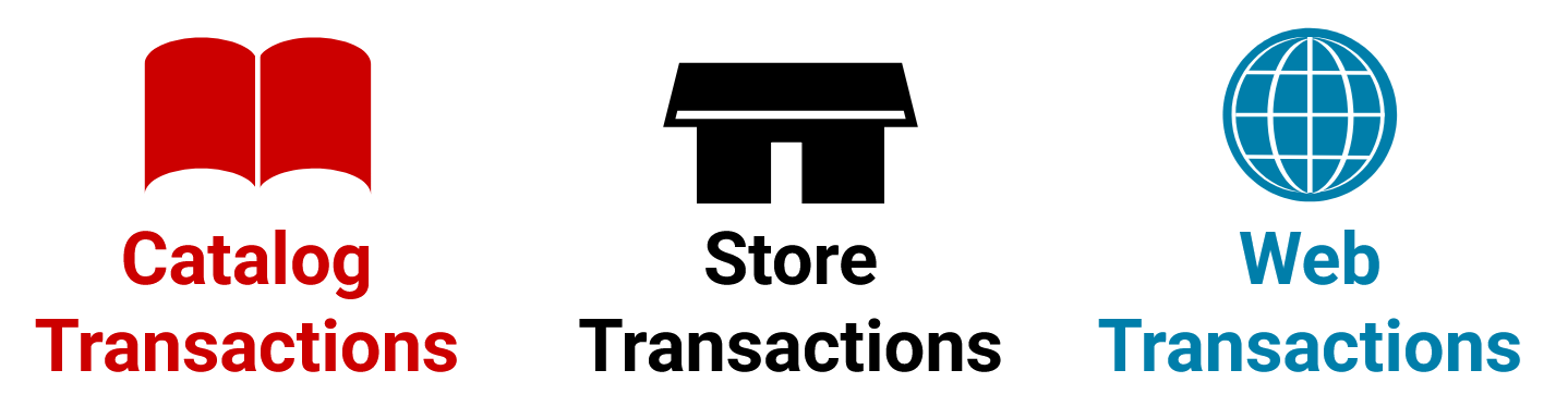
Each type of sale is stored within the CATALOG_SALES, STORE_SALES and WEB_SALES Tables held on the Snowflake TPC-DS data store. Each sale type also has associated returns, which are stored within the CATALOG_RETURNS, STORE_RETURNS and WEB_RETURNS Tables respectively. These Tables contain transactions on a one-sale, one-row basis.
Associated details of the sale, such as the item that was sold (CS_ITEM_SK) or the net price that was paid (CS_NET_PAID) are each columns of the Table. Each column of each table is labeled with a prefix (e.g. CS_) which is an abbreviation of the Table name, meaning that all the columns across all the Tables have unique identifiers. In many cases, columns will refer to a surrogate key (_SK) which corresponds to a foreign key in another Table.
Examples of other, non-transaction Tables are the CUSTOMER or ITEM Tables. These contain (predictably!) additional information about all the customers and items that are involved in the transactions. An example of a foreign key link would be that SR_CUSTOMER_SK column of the STORE_RETURNS Table corresponds directly to the C_CUSTOMER_SK column of the CUSTOMER Table. Within your relational data store, you would use these keys to query information across Tables. They will also be a key component of our graph construction.
The specification document linked above outlines the entire schema of all the Tables in the TPC-DS dataset, and specifies precisely which columns of individual tables link to other tables via foreign keys. The TPC-DS dataset is large and rich, meaning we have a number of options for how to convert all this information into a graph. To avoid getting too bogged down in analysis paralysis, however, let’s start simple.
Creating Nodes
First, let’s begin with the transactions themselves. We will simply model each individual sale and return (i.e. each row of the sale and return Tables) as a straightforward node: CatalogSale, CatalogReturn, StoreSale, StoreReturn, WebSale and WebReturn.
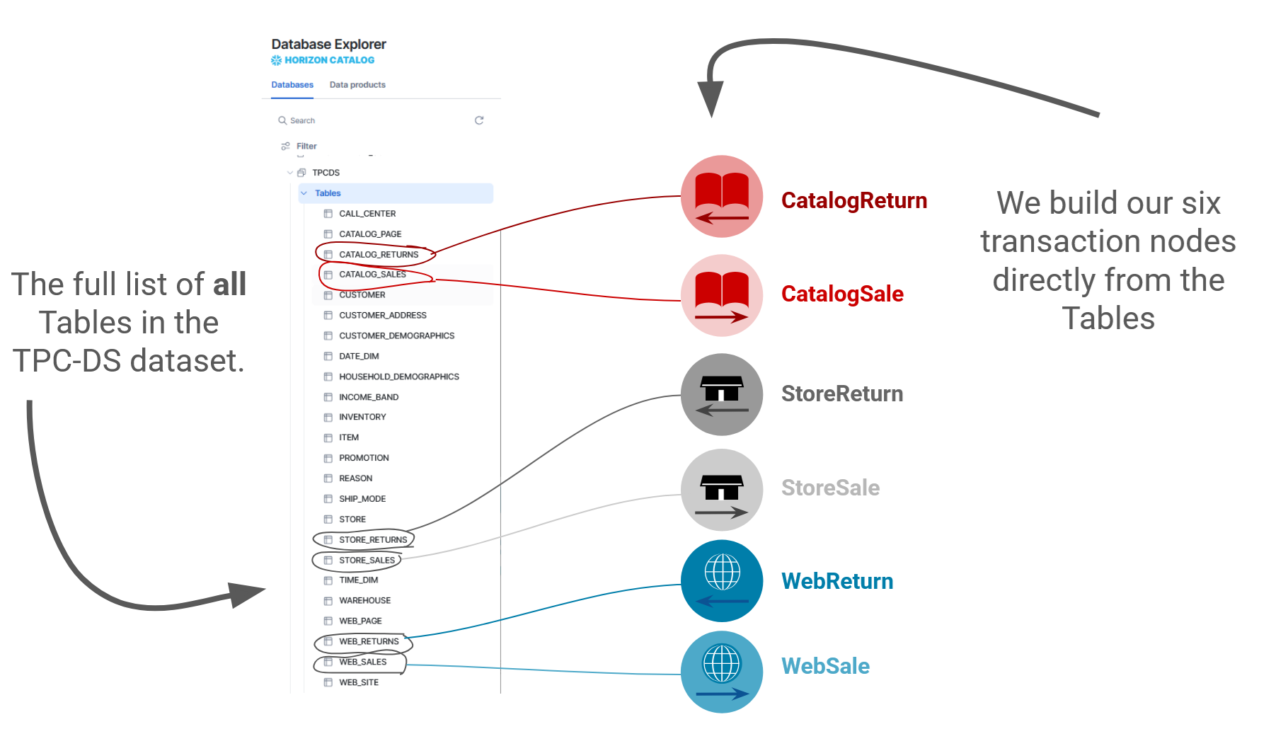
Within LadybugDB we define a node by first creating a NODE TABLE with name NodeName. We also assign it a primary key and whatever properties we would like to add:
CREATE NODE TABLE IF NOT EXISTS NodeName (id STRING PRIMARY KEY, property1 STRING, property2 INT64, etc . . . )
(Note that we drop the conn.execute() here, but it’s implied). We then populate the NODE TABLE by using the COPY functionality, which will transplant the results of a wrapped SQL query into our table:
 COPY NodeName FROM (
        LOAD FROM [SOURCE]
        RETURN ID_COLUMN, PROPERTY_COLUMN1, PROPERTY_COLUMN2, etc . . .
    );
In the case of our transaction nodes, we will model each column of the corresponding Tables as a property. For example, we will model the columns of CATALOG_SALES which have names like CS_BILL_ADDR_SK, CS_BILL_CDEMO_SK, CS_BILL_HDEMO_SK etc. as properties of our CatalogSale node with the form bill_addr_sk, bill_cdemo_sk, bill_hdemo_sk etc.. You can extract the column names of any given Table by using the get_column_names() function:
def get_columns(table_name):
    result = conn.execute(
        f"""
        LOAD FROM sf.{table_name}
        RETURN * LIMIT 1 ;
        """)
    columns = result.get_column_names()
    return columns
From here you can straightforwardly use Python to both loop over the names of the existing columns, and construct new node properties names you want to use. Assuming you want just want to convert each single column directly into a single new property, then you can simply reuse the names .
The one exception is the node primary key itself. Because each individual sale does not in itself have a unique key, it can only be uniquely identified by the combination of its item number {}_ITEM_SK and order or ticket number {}_ORDER_SK/{}_TICKET_SK. This is detailed in Section 2 of the specification document, where transactions are always shown with both order and item foreign keys cited as the primary key.
To account for this, we cannot simply return the order number or the ticket number individually, we have to return a composite key constructed from both as the primary key. Fortunately, this is easy to do: string(CS_ORDER_SK) + '_' + string(CS_ITEM_SK)
The complete LadybugDB functionality to create our first CatalogSale node is then:
CREATE NODE TABLE IF NOT EXISTS CatalogSale (id STRING PRIMARY KEY, bill_addr_sk INT64, bill_cdemo_sk INT64, bill_customer_sk etc . . . )

RETURN string(CS_ORDER_SK) + '_' + string(CS_ITEM_SK) AS composite_key, CS_BILL_ADDR_SK, CS_BILL_CDEMO_SK, CS_BILL_CUSTOMER_SK, ....
(Where I’ve omitted the full list of properties for brevity.)
If you’ve followed so far, then the rest of the node creation is even easier. Similarly, we also directly convert the CUSTOMER, ITEM, PROMOTION, REASON, WAREHOUSE and WEB_SITE Tables into Customer, Item, Promotion, Reason, Warehouse and Website nodes respectively. In this case, each row of these Tables does have a unique surrogate key, so we simply use this as the node primary key and do not have to define any composite key.
N.B. LadybugDB does not allow any two TABLE objects to share the same name, and that table names are case insensitive, so you may need to slightly alter names to avoid clashes between your node tables and Snowflake tables, such as using CustomerNode instead of Customer.
Creating Edges
But of course no graph is complete with only nodes, so let’s consider the relationships in our data. Fortunately, the creators of the TPC-DS dataset already appreciated graphs, because the specification document includes entity-relationship (graph) diagrams modeling the connections between different Tables. We can refer to an example of the WEB_SALES Table shown in the Web Sales ER-Diagram (Figure 2.3.5.1) of the specification document:
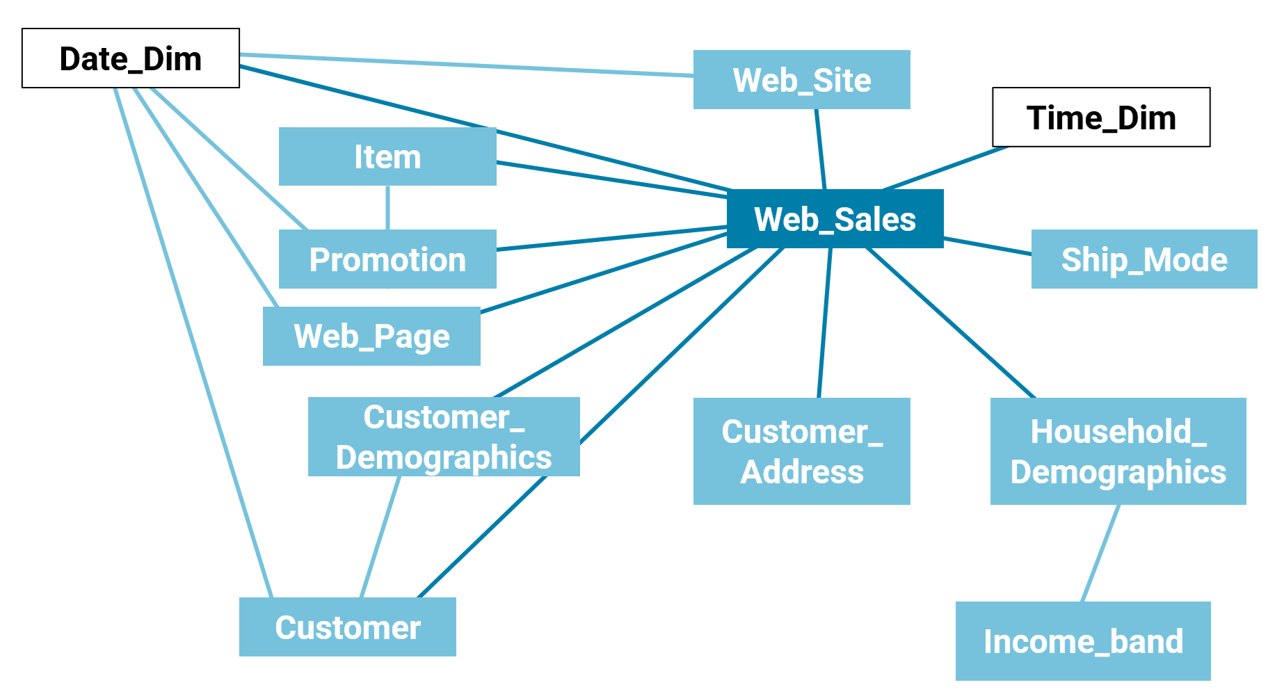
The edges in this diagram correspond to cases where there is a simple link between two Tables via a foreign key, as we discussed before. Since we have simply modeled most of our Tables directly as nodes, it makes sense that to use these predefined links to model our edges in a similar way.
Creating an edge in LadybugDB is very similar to creating a node. Instead of creating a NODE TABLE, we create a REL TABLE between two existing types of NODE TABLE:
CREATE REL TABLE IF NOT EXISTS EdgeName (FROM NodeName1 TO NodeName2, property1 STRING, property2 INT64, etc . . . )
And then once again we populate the edge by using the COPY command.
    COPY EdgeName FROM (
        LOAD FROM [SOURCE]
        RETURN DISTINCT ID_COLUMN1, ID_COLUMN2, PROPERTY_COLUMN1, PROPERTY_COLUMN2, etc . . .
    )
Since our simple edges are currently defined as nothing more than the link between two Tables via foreign keys, we probably don’t need to attribute them with any properties at the moment.
Note also that, in LadybugDB, a REL TABLE is defined by the two NODE TABLES that it links, and that LadybugDB does not allow two REL TABLE entities to share the same name. This means that you cannot, for example, have both the CatalogSale and WebSale nodes link to Item nodes via sold_item edges. Instead, all edges must have unique names, e.g. cs_sold_item and ws_sold_item.
Remembering that transactions are identified by composite primary keys, our code to create an edge will then look something like this:
    CREATE REL TABLE IF NOT EXISTS ws_sold_item(FROM WebSale TO Item)
    COPY ws_sold_item FROM (
        LOAD FROM sf.WEB_SALES
        RETURN DISTINCT
        string(WS_ORDER_NUMBER)+'_'+string(WS_ITEM_SK),
        WS_ITEM_SK
    );
More Complicated Properties
You may have noticed in the ER diagram above that I coloured the time (‘Time_Dim’) and date (‘Date_Dim’) entities in white. The reason for that is that these Tables are a little different. The rows of the DATE_DIM and TIME_DIM Tables don’t really correspond to any distinct objects or concepts in the same way the CUSTOMER or ITEM Tables do. Instead, they contain a complicated mapping that turns codes representing the date and time (surrogate keys) into the actual times and dates as humans would understand them.
This is the kind of thing which might be preferable for traditional relational data querying, but could look really quite strange if we tried to map every individual time and date stamp to an individual node on our graph. We’d still like to include this information (temporal data is pretty important for analysing real-time transactions!) but we’d like to include it in a form that’s human-readable for our graph.
Fortunately, this is also a great way to demonstrate how you can do something a little more complicated with your data. Instead of just directly mapping these Tables to Nodes or Edges, we’re going to extract, cross-reference and manipulate the data from a Table to augment an existing Node.
We use LadybugDB to extract all the information we need from e.g. the WEB_SALES, TIME_DIM and DATE_DIM Tables, then we use python to merge them all together into a single dataframe store. From here, we can look up the WS_SOLD_TIME_SK column in the first Table. We check it against the TIME_DIM Table and extract the T_HOUR, T_MINUTE and T_SECOND columns. We compile and transform data from this columns into a new string with a HH:MM:SS format and store it as a new time property. We can then do the same process again for the date:
    # Define the WebSale node
    conn.execute(f"CREATE NODE TABLE IF NOT EXISTS WebSale(id STRING PRIMARY KEY, date STRING, time STRING)")

    # Load store sales as a dataframe
    ws_result = conn.execute(f"""
        LOAD FROM sf.WEB_SALES
        RETURN DISTINCT {original_properties}
    """).get_as_df()

    # Load time details as a dataframe
    t_result = conn.execute("""
        LOAD FROM sf.TIME_DIM
        RETURN T_TIME_SK, T_HOUR, T_MINUTE, T_SECOND
    """).get_as_df()

    # Load date details as a dataframe
    d_result = conn.execute("""
        LOAD FROM sf.DATE_DIM
        RETURN D_DATE_SK, D_DATE
    """).get_as_df()

    # Merge everything into a single dataframe
    # Merge the data from WEB_SALES and TIME_DIM, by matching the 'WS_SOLD_TIME_SK' column to the 'T_TIME_SK' column
    merged = ws_result.merge(t_result, left_on='WS_SOLD_TIME_SK', right_on='T_TIME_SK')
    # Do the same for the date
    merged = merged.merge(d_result, left_on='WS_SOLD_DATE_SK', right_on='D_DATE_SK')

    # Populate the node
    # Date is provided in YYYY-MM-DD format by default
    # We reformat the time to HH:MM:SS format
    conn.execute(f"""
        COPY WebSale FROM (
        LOAD FROM merged RETURN
        string(WS_ORDER_NUMBER) + '_' + string(WS_ITEM_SK) AS composite_key,
        to_string(D_DATE),
        lpad(to_string(T_HOUR), 2, '0')+':'+lpad(to_string(T_MINUTE), 2, '0')+':'+lpad(to_string(T_SECOND), 2, '0'))
        """,
        {"merged": merged}
        )
What this demonstrates is how much flexibility you have when extracting your data in LadybugDB. You have everything from your existing Snowflake graph store at your fingertips, and you get to choose how you build your graph from that.
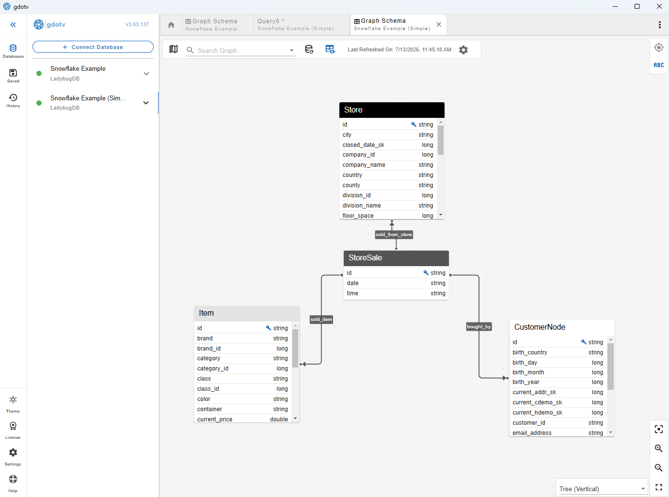
Here’s a data model that illustrates a concept from each step we’ve tried so far. The Store, Item and Customer nodes have been imported directly with a simple column-to-property conversion from the STORE, ITEM and CUSTOMER Tables, the sold_from_store, sold_itm and bought_by edges have been constructed from foreign key links between Tables, and the StoreSale node has been created from the STORE_SALES Table, with the new date and time properties that we just constructed from the TIME_DIM and DATE_DIM Tables.
But we don’t want to have a sales node with only date and time properties, so we convert all the others in the same way as above.
That leaves us with a node that contains all the columns of the original, with additional time and date properties, as below:
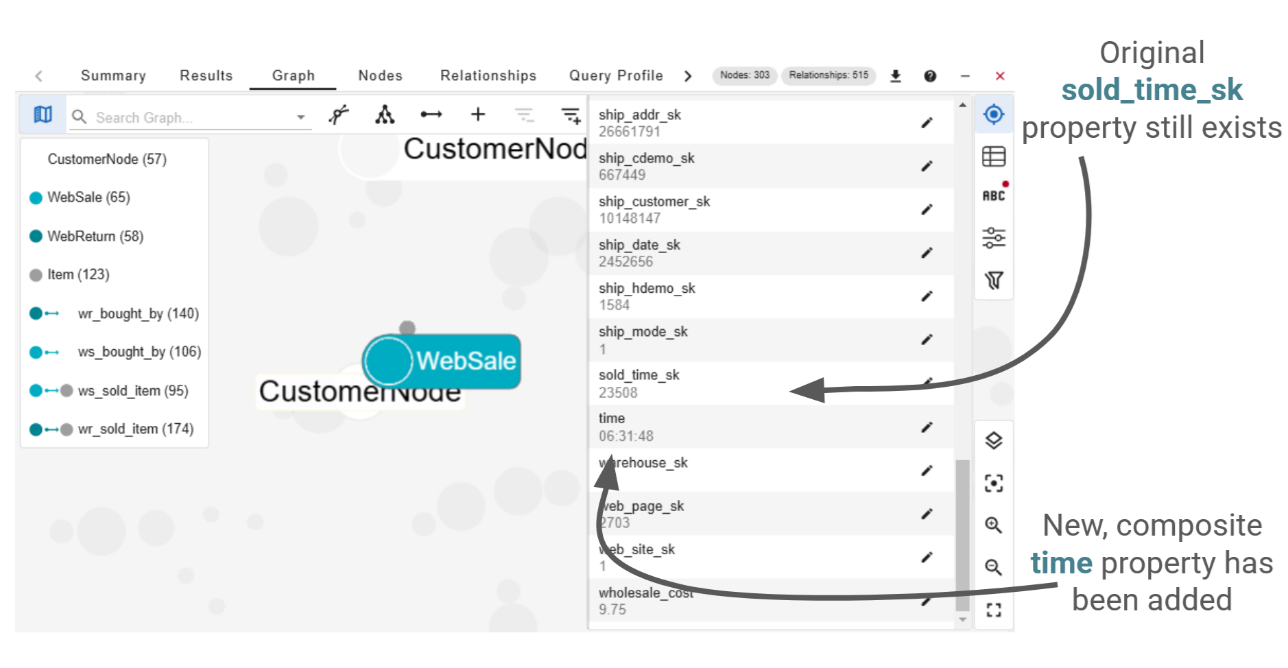
Further Discussion: This approach of transferring all the original columns over as properties and adding more properties on top means that you maintain complete preservation of the original data within your graph. However, it’s also somewhat redundant, since it’s unlikely you would ever want to consult the sold_time_sk property if you already have already created the more directly useful time property. So you may wish to omit copying the former property into your node altogether. On the other hand, you may wish to preserve it for validation.
Making these kinds of choices (when to preserve, transform or remove data) is part of the art of knowledge graph creation. Making them well is the real skill of being a knowledge graph engineer. And what determines a good choice really depends on what you’re planning to use your knowledge graph for.
Since you’ll likely still have access to your original relational data store, you may find that copying every single column of data over on a 1:1 basis is not the best way to leverage graph technology against your database. Often, the best new insights come from reshaping your data entirely to new forms. Constructing composite entities and properties lets you make connections across your graph that you might not have otherwise seen.
With the philosophical discussion out the way, let’s add in a series of additional nodes, and all the other properties. From here, we can get an overview of the graph from looking at the gdotv Data Model view.
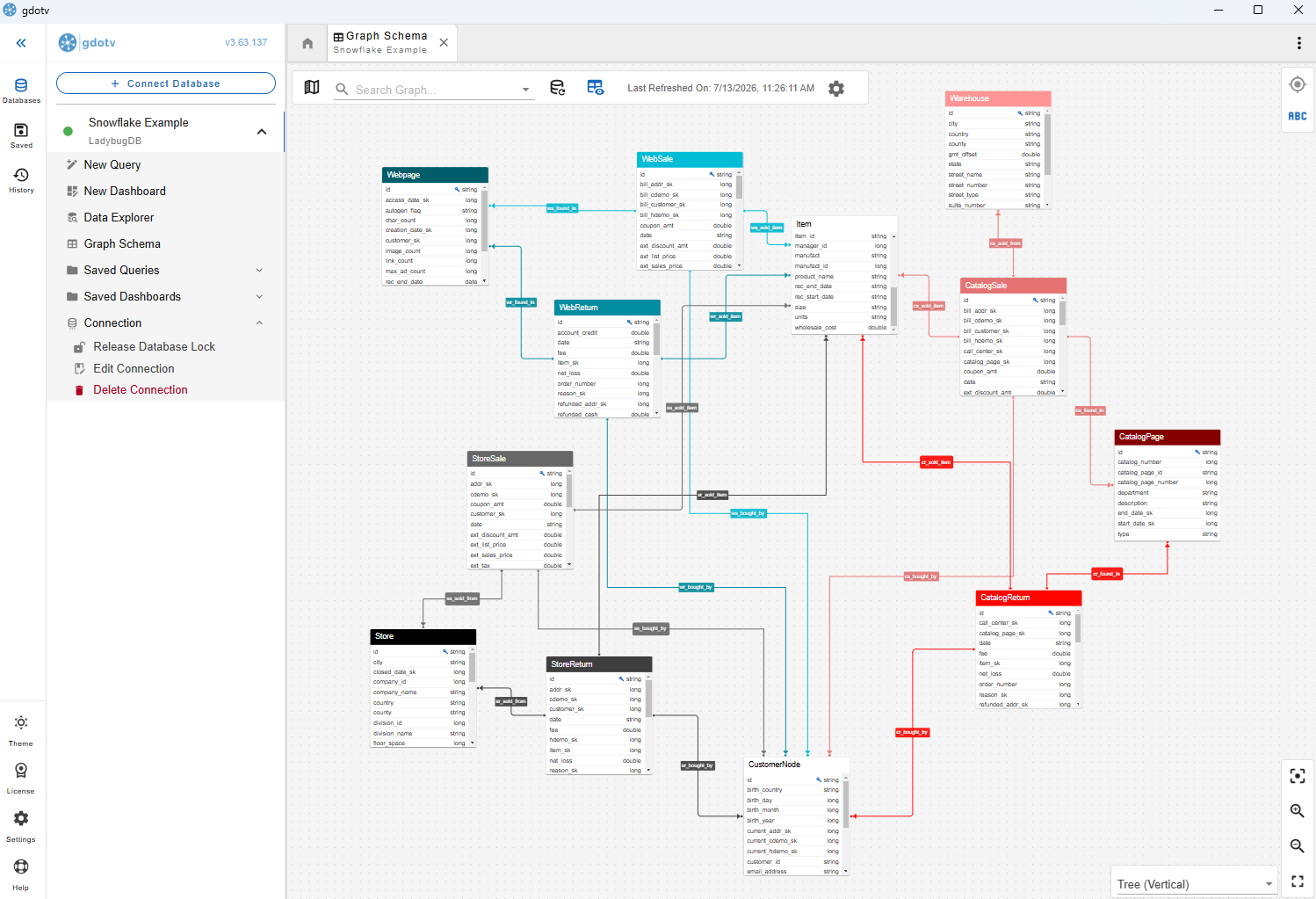
One of the nice things about gdotv’s intuitive UI is that it gives you a number of customization options to help you get a clearer view of what’s going on. In this case, since the graph is loosely composed into three types of sale, I’ve customized the nodes and edges with a matching colour scheme. Entities related to Stores, Catalogs and Webpages are coloured black, red and blue respectively. We also have the ‘neutral’ Item and Customer nodes which can be part of any sale, so I’ve coloured those in white.
Note that I’ve included most of the information from the TPC-DS dataset, but not all of it. There are additional Tables, such as the DEMOGRAPHICS, PROMOTION and INCOME Tables, which I have omitted just to keep the graph fairly compact and readable. These Tables contain useful additional information about the Customer and Item nodes. You could do all kinds of things with this information. We have focused on the ‘sale’ aspect of the transactions so far, but the TPC-DS dataset also includes rich demographic information that changes in time, as customers do not necessarily stay part of the same income band, for example. You could envision an entirely different form of the graph that focuses on this aspect instead.
Exploring with gdotv
While building your graph, you might want to take a look at the data itself. This can help you see what kinds of nodes and edges will be most useful to you. For any LadybugDB dataset, you can query your data with Cypher in the gdotv query editor. Cypher is produced by Neo4j, and you can read their tutorials here. gdotv also has built-in documentation, schema-aware autocomplete suggestions and syntax highlighting available for Cypher, to help make querying as easy as possible.
If you’re not a fan of writing code, though, gdotv also has a couple of no-code options available. My favourite is the Data Explorer. This lets you search for paths with a given structure within your graph, no querying necessary. You can even apply filters to your search.
Let’s do an initial check for paths that match Item nodes with the category property category = 'Books'. We’d like to know where customers are finding books, so let’s also check for which CatalogPage are associated with these books.
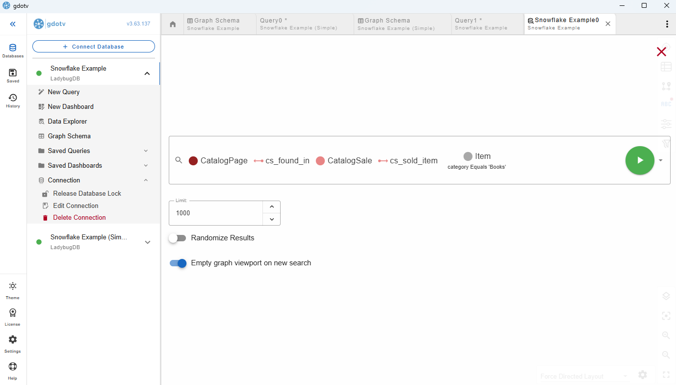
We get out the following graph.
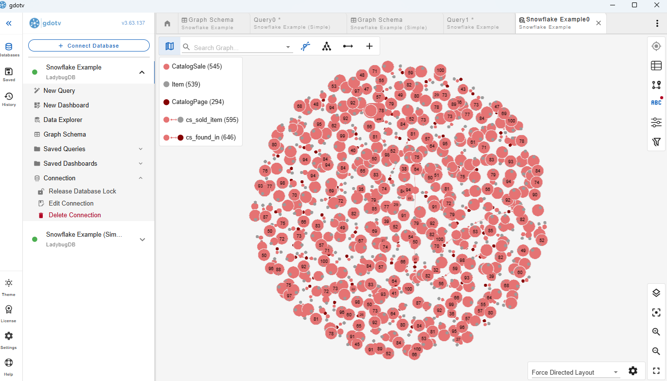
At first glance, it’s messy, and doesn’t seem to tell us much about where users are finding these products.
First impressions aren’t always correct, however, so let’s take a closer look. We start by setting custom labels for our CatalogPage nodes that depend on the catalog_number and catalog_page_number properties:
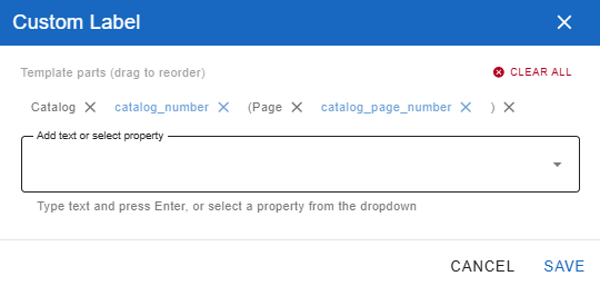
This is just to make it easier to see what’s going on. Now we zoom in closer on the graph:
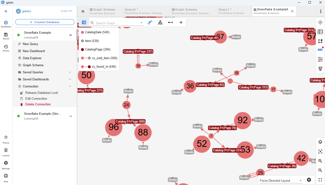
As we can see, many of these CatalogPage nodes actually come from the same catalog, number 91. Unfortunately, that’s difficult to tell here, because the catalog_number is still just a property of the Catalog node. There’s nothing (other than our eyes and brain) telling us that these are actually referring to the same catalog.
The issue is that we lifted our catalog information directly from the CATALOG_PAGE Table in our dataset stores, applying only the most basic conversion (i.e. turning every row into a node). This is sufficient for some entities, like turning our CUSTOMER Table into our CustomerNode nodes, but because CATALOG_PAGE contains pages from all the catalogs in one central dataset, the graph doesn’t do a great job of revealing which CatalogPage nodes belong to the same Catalog. We could simply query against this property, but we would better leverage graph capabilities by modeling this relationship explicitly.
To do this, we now make a new Catalog node from the distinct entries in the CATALOG_NUMBER column.
CREATE NODE TABLE IF NOT EXISTS Catalog(id STRING PRIMARY KEY)

COPY Catalog FROM (
        LOAD FROM sf.CATALOG_PAGE
        RETURN DISTINCT CP_CATALOG_NUMBER
        )
We also make a part_of_catalog edge which links our CatalogPage and Catalog nodes. If we rerun our search, we can far more easily see both the impact of Catalog 91, and also which of its pages are connected with the highest number of CatalogSale nodes:
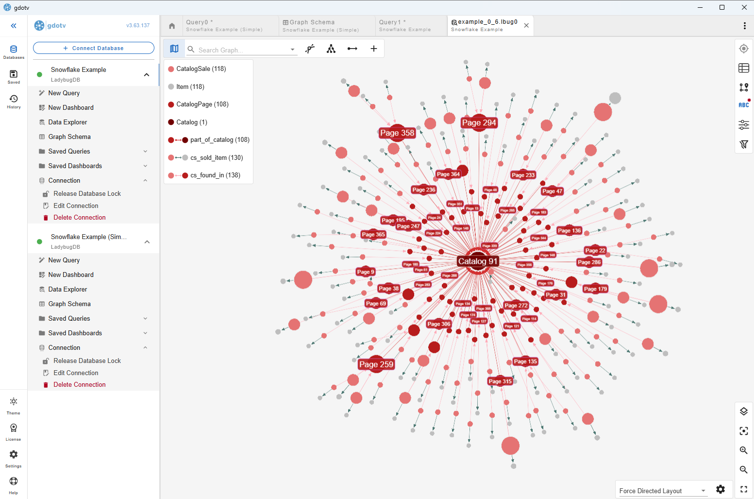
This is the real power of graph-on-relational functionality. Once we’ve structured our graph to look for the relationships that interest us, a new significant connection immediately jumps out the page.
Of course, even now this is just one way to implement connectivity across relational Tables into your LadybugDB graph. Here, we have just done the most basic fix. We have added a new node and edge, while preserving the existing structure of the graph. (Similar to how we just added a property before, without removing any existing properties).
But if, for example, you were not terribly interested in graphing exactly which pages correspond to which sales, then you could eliminate the CatalogPage node entirely, and instead model the page number as a property of a direct cs_found_in edge between CatalogSale and Catalog nodes. Again, it all depends on which parts of your data you want to model.
Conclusion
There we have it, a walkthrough of just a few things to think about when using a relational data store to build your first LadybugDB database. It’s so exciting that LadybugDB have added ADBC compatibility, making it easier than ever to turn data from Snowflake and other vendors into graphs.
If you’d already built your graph and want to know more about how you can query, modify and explore the data itself with gdotv, check out our companion page on LadybugDB. You can even see my video where I walk you through the basics! Whether your graph is finished or not, you should consider gdotv as a useful tool in your kit. Why not download a free trial to see what gdotv can bring to your LadybugDB experience?
That’s all from me, good luck!