Visualizing Apache AGE: Connecting gdotv and Exploring the Air Routes Graph

You have an Apache AGE instance running, with either the air routes dataset from the previous post loaded or a graph of your own you’d like to look at. The next question is how you actually look at it. Cypher in psql works, but graphs reward visual exploration in a way tables don’t. Switching between “write a query” and “see what’s there” is where a graph-aware client earns its keep.

This post walks through connecting gdotv to your AGE instance and exploring the graph: schema discovery, Cypher editor, visualization, and interactive neighbor expansion. It also touches on a couple of AGE-specific behaviors gdotv handles for you, like AgType deserialization and the cypher() SQL wrapper. The screenshots show the air routes dataset, but everything described works the same against any AGE graph.

This is the final part of a 4-post series on Apache AGE.

Setup assumptions

This post assumes you have:

• An Apache AGE instance running, either locally via the Docker setup from part 2 of this series or on a managed cloud Postgres provider that supports AGE.
• A graph with some data in it. We’ll reference the air_routes graph from part 3 of this series throughout, but if you have your own AGE graph loaded with data already, swap it in mentally as you go: the workflow is the same, only the label and property names change.
• gdotv installed. It’s available at gdotv.com and runs on macOS, Windows, and Linux.

Connecting gdotv to AGE

In gdotv, start a new connection and pick Apache AGE from the database list.

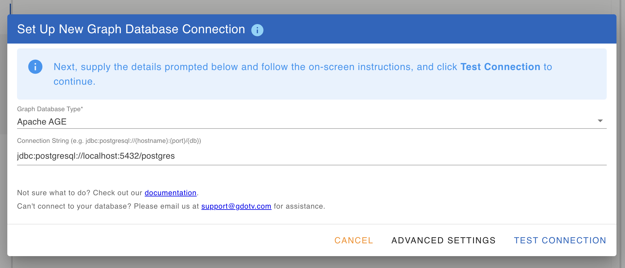
The connection details mirror a standard Postgres JDBC connection:

• JDBC URL: jdbc:postgresql://localhost:5432/postgres for the local Docker setup. For cloud Postgres, paste in the JDBC URL your provider gives you.
• Username / password: postgres / password for the local Docker setup. For Azure-hosted AGE, you can switch to Microsoft Entra ID authentication: For Azure for PostgreSQL only – to configure Entra ID authentication via the Azure CLI to leverage your Azure PostgreSQL Entra ID temporary user credentials.

Once the connection details are in, gdotv runs an auto-detect step before saving. It probes ag_catalog.ag_graph to confirm the AGE extension is actually enabled, lists the available graphs on that database, and surfaces actionable guidance if anything’s off (extension not installed, credentials missing, hostname unreachable, and so on).

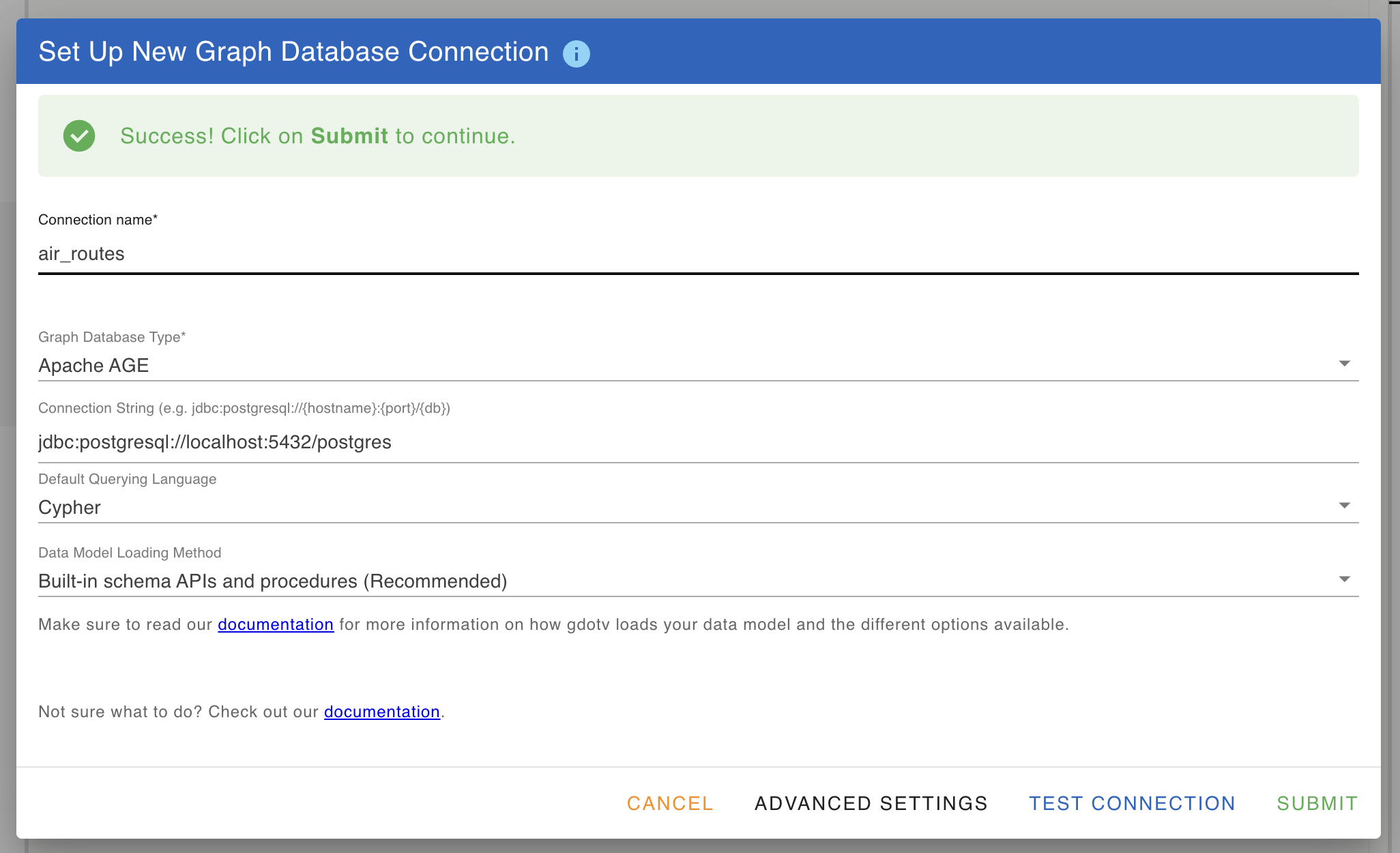
Pick the air_routes graph (or your own) and save the connection. The per-session LOAD 'age' and search_path setup that AGE requires are run automatically on every new connection, so you can jump straight to writing Cypher.

The Cypher (and SQL) editor

Switch to the query editor to start writing (and running) Cypher queries.

A few things gdotv does behind the scenes here:

• No SQL wrapping required. AGE’s Cypher dialect is normally invoked through a SELECT * FROM cypher('graph_name', $$ ... $$) AS (col agtype) SQL wrapper. In the editor, you write plain Cypher; gdotv injects the wrapper, the graph name, and the agtype column aliases for you.
• Parameters as native Cypher params. Use $paramName references in your Cypher; gdotv collects parameters from the parameters panel and sends them through as a single AgType map (which is the only parameter shape AGE accepts). You don’t need the prepared statement + USING ... dance manually.
• Autocomplete for labels, property keys, and Cypher keywords, derived from the schema view above. If a label or property key isn’t showing up in suggestions, the schema sample probably hasn’t seen it yet; refreshing the schema picks it up.

Cypher covers the graph-shaped questions cleanly, but it’s not the only thing you’ll want to run. AGE sits inside a regular Postgres database, and the more interesting queries often combine the two: a Cypher pattern joined against a regular relational table, an aggregate that pulls vertex properties into a GROUP BY, or a COPY into a staging table à la part 3.
gdotv treats SQL as a first-class query language alongside Cypher: you can write and run plain SQL (including the cypher(...) form yourself if you want full control), with the same result handling on the way back: the same typed property panel, the same table view, and graph rendering for any rows that come back as vertices, edges, or paths. The point is that you’re not stuck switching to a separate tool the moment your question stops being purely graph-shaped.

Schema view

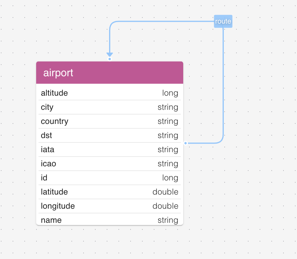
Before moving on to graph visualization, let’s take a quick look at the schema view. It’s there to show you every vertex and edge label in your graph, the properties on each, the types of those properties, and how the labels connect to one another.

A few things the schema view is particularly useful for:

• A shared mental model of the data, for you and your team. Everyone connecting to the same graph sees the same labels, properties, and types in the same shape. New team members can be brought up to speed on what’s in the graph without a Confluence page or a one-on-one walkthrough; the panel itself is the documentation.
• Onboarding to an unfamiliar graph. If you’ve inherited an AGE graph from someone else, the schema view is the fastest way to see what’s actually in there without writing exploratory queries.
• Confirming a load went the way you expected. After running through part 3 of this series, the schema view is where the difference between an agload-style load and a staging-table load shows up most clearly: property types either look right at a glance, or they don’t.
• Powering autocomplete and validation in the Cypher editor. As you type a query, gdotv autocompletes label and property names from the schema, and warns about references that don’t exist (a typo’d label, a property that isn’t on the matched vertex). That feedback loop closes a class of “ran the query, got zero rows, didn’t notice the typo for ten minutes” mistakes that happen on a flexible-schema graph more than they should.

AGE itself doesn’t enforce a strict schema (it’s the same flexible-property model as most property-graph engines), so the schema view is non-strict by design — you can add new labels and properties at any time just by writing a Cypher CREATE, and refreshing the schema picks them up.

Graph visualization

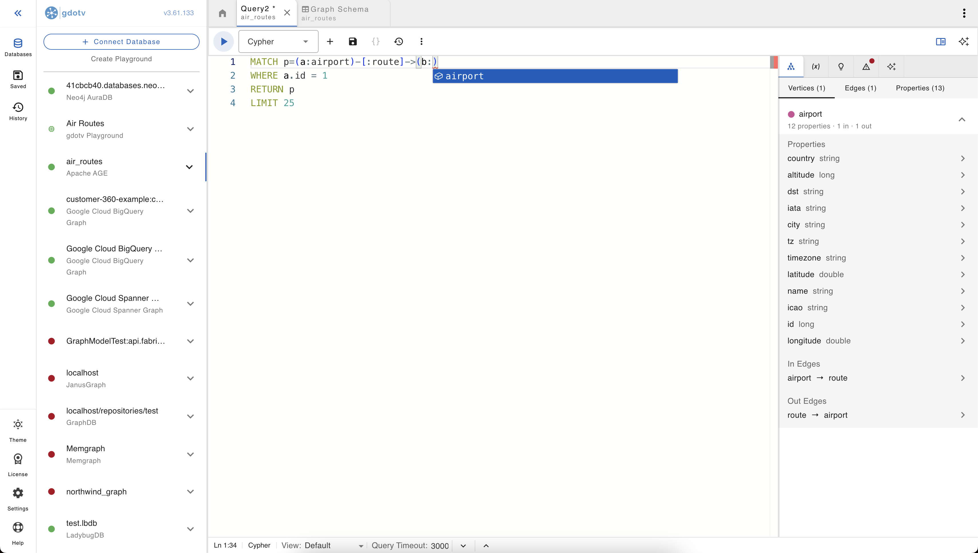
When a query returns vertices or edges, gdotv renders them automatically as a graph, on top of offering regular table views. Pattern-returning queries (those returning a p from MATCH p=...) are particularly useful, since the entire matched path lights up.

For example, pick any airport from the dataset and pull its outbound routes:

MATCH p=(a:airport)-[:route]->(b:airport)
WHERE a.id = 1
RETURN p
LIMIT 25

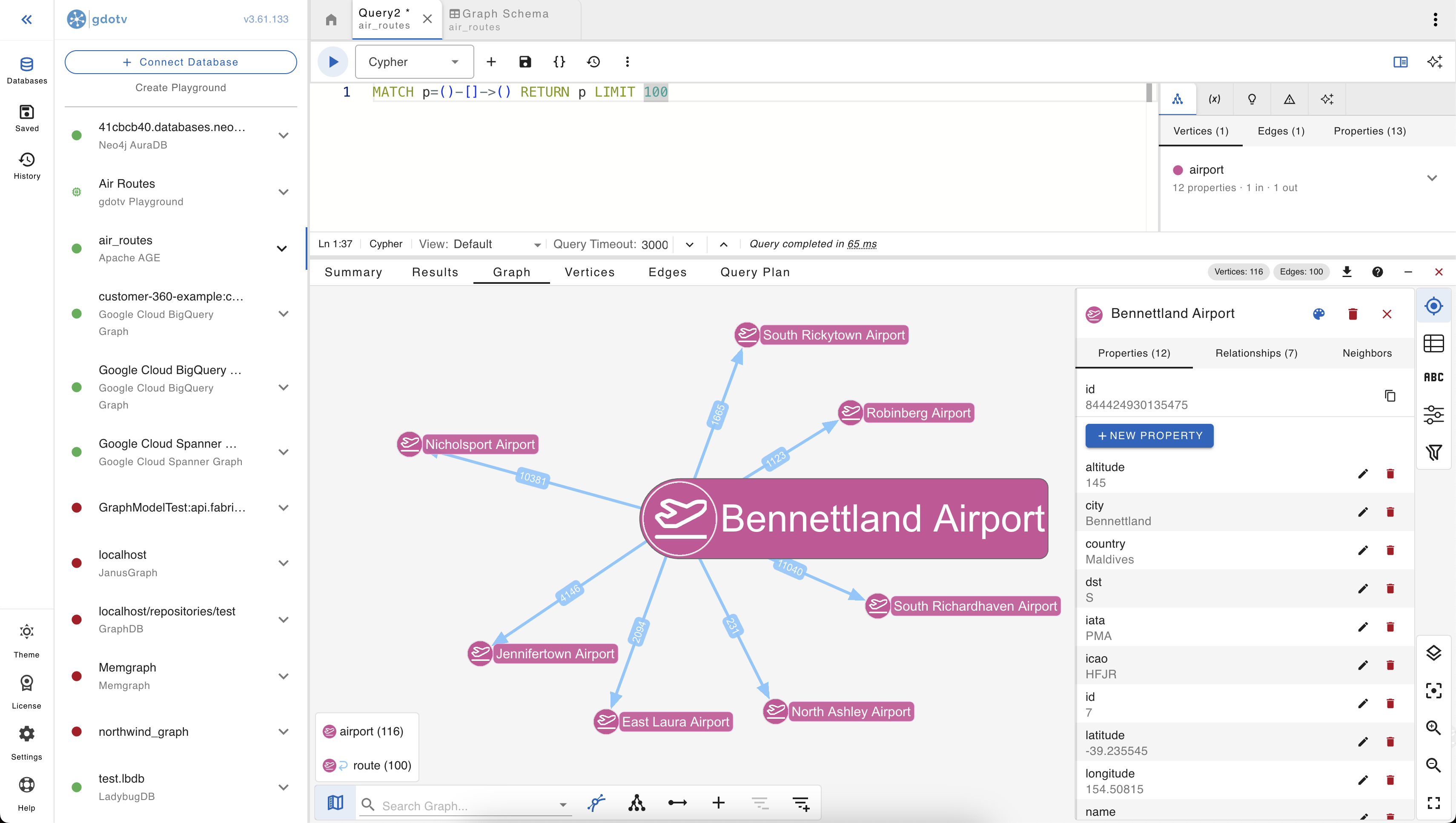
Some details worth pointing out:

• Vertex colors and edge colors are assigned per label, automatically. With only airport and route in this graph, the visualization is two-tone; richer schemas pick up more of the palette.
• Edge directionality comes through (the arrowhead points from the start vertex to the end vertex), which matters for asymmetric route data.
• Hovering or clicking a vertex/edge surfaces its properties in a side panel, with values typed correctly (numbers as numbers, strings as strings) rather than as raw AgType blobs.

Interactive neighbor exploration

Once you have a few vertices on the canvas, you can expand outward by clicking a vertex and asking gdotv to load its neighbors. This is where graph exploration starts feeling fundamentally different from running ad-hoc queries: you follow your curiosity rather than pre-shaping it into a MATCH pattern.

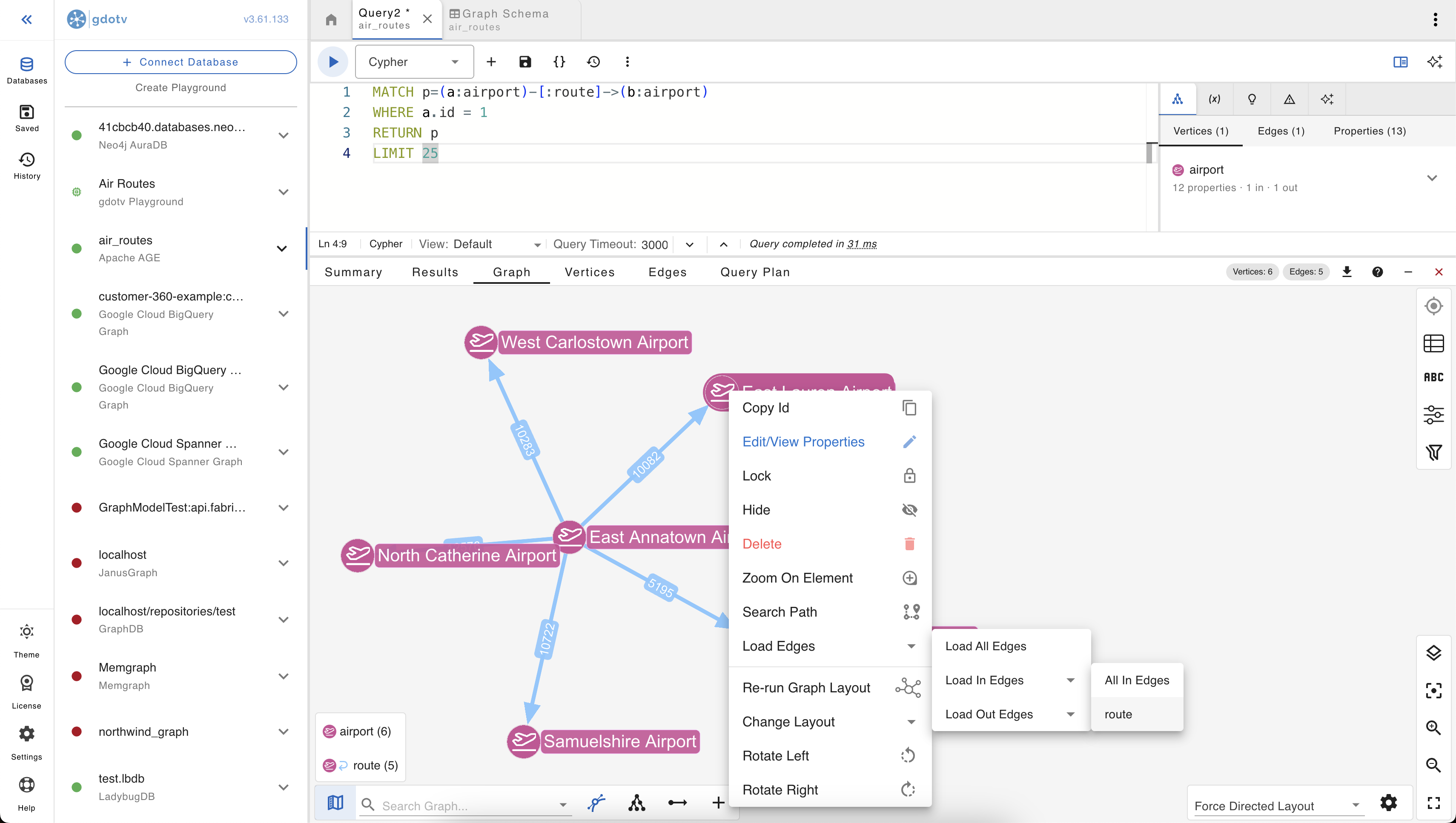
Expansion respects edge direction: separate “expand outbound”, “expand inbound”, and “expand all” actions on each vertex. Useful in a directed graph like air routes where the inbound and outbound neighborhoods of an airport are different sets and you usually only want one or the other.

The no-code graph explorer

The expand-from-a-vertex flow above is part of a broader no-code explorer in gdotv. Instead of writing Cypher, you start from a label or a specific vertex, then build the query up visually: pick a starting label, add filters on properties, follow edges out (or in), filter again, choose what to return. Each click adjusts the query gdotv runs underneath, and the visualization updates in place.

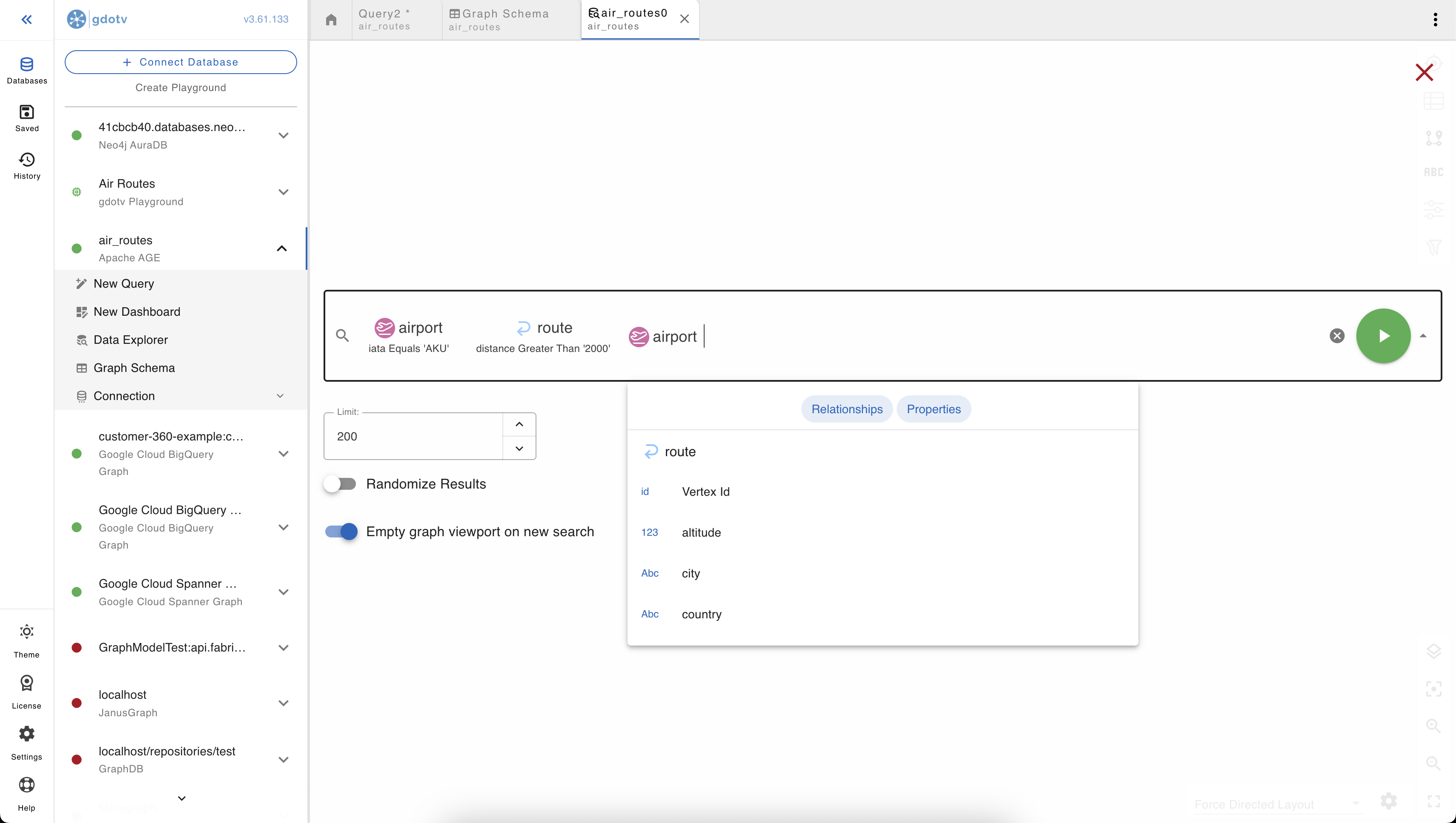
Once a path and its filters are specified, gdotv automatically generates and runs a Cypher query for it. You can switch over to the editor at any point to see the underlying query, copy it out, modify it, and run it back. That makes the no-code explorer useful in a couple of distinct modes:

• Genuinely no-code exploration, for analysts and stakeholders who want to ask questions of the graph without learning Cypher.
• A starting point for a query you’d otherwise have to write from scratch. Build the rough shape visually in a few clicks, switch to the editor, and refine from there. Faster than typing a MATCH chain by hand, especially against an unfamiliar schema.

A guided tour of the air routes graph

A few queries to get a feel for the dataset.

1. Find an airport by IATA code:

MATCH (a:airport {iata: 'AKU'})
RETURN a

The synthetic dataset uses real-looking IATA codes, but the airport names and cities are generated. Use the IATA code as the lookup key; the names won’t be familiar.

2. Find the airports with the most outbound routes:

MATCH (a:airport)-[:route]->()
RETURN a.iata, a.city, count(*) AS outbound
ORDER BY outbound DESC
LIMIT 10

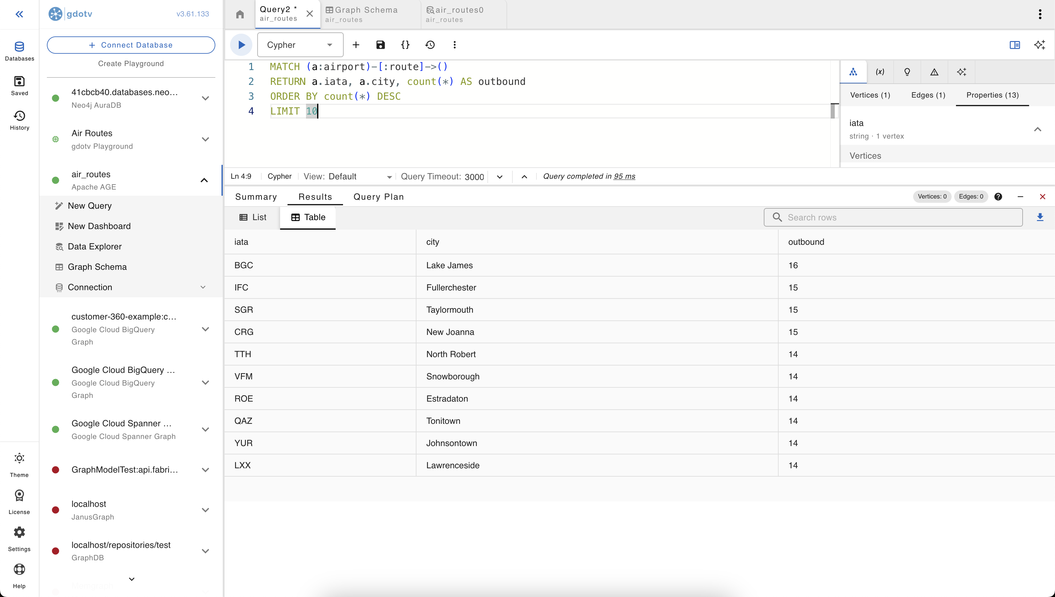
This one’s a good reminder that graph visualization does not have to be the default view for a graph query. Sometimes we just need a good old table to quickly compare results.

3. Two-hop reachability from a starting airport:

MATCH p=(a:airport {IATA: 'AKU'})-[:route*1..2]->(b:airport)
RETURN p
LIMIT 100

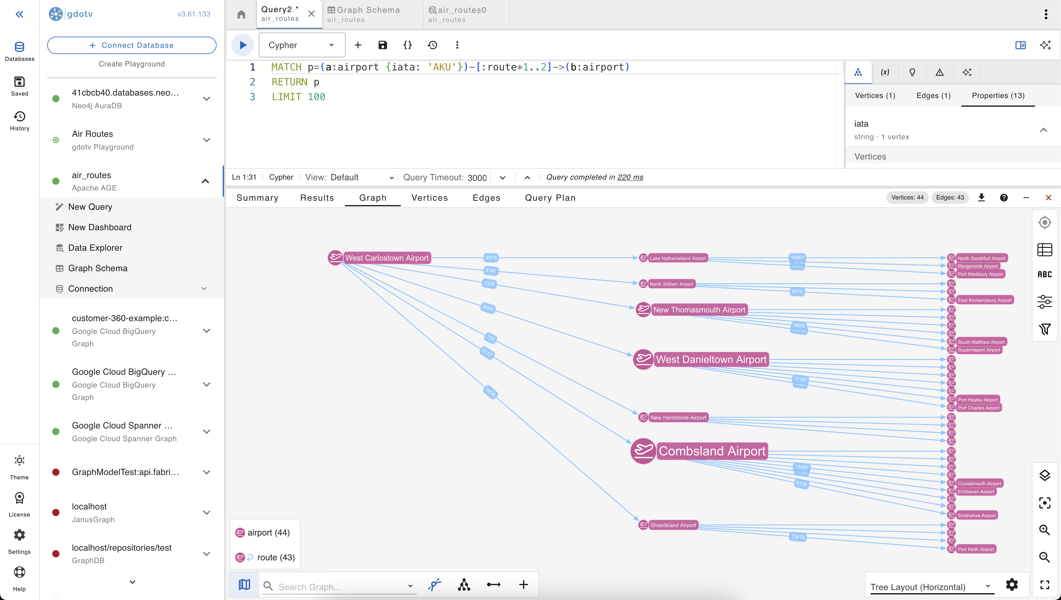
This is the kind of query that’s awkward to read as a table and intuitive to read as a visualization. The pattern variable [:route*1..2] matches paths of length 1 or 2; gdotv renders each path as a chain on the canvas, and overlapping chains share their vertices automatically.

Editing data: vertices, edges, and properties in-place

What if you just want to make a small tweak to the data quickly? Fix a misspelled property, add a missing edge between two airports, drop a stray vertex that shouldn’t be there. gdotv has a WYSIWYG data editor that lets you do those changes directly from the visualization, no Cypher required.

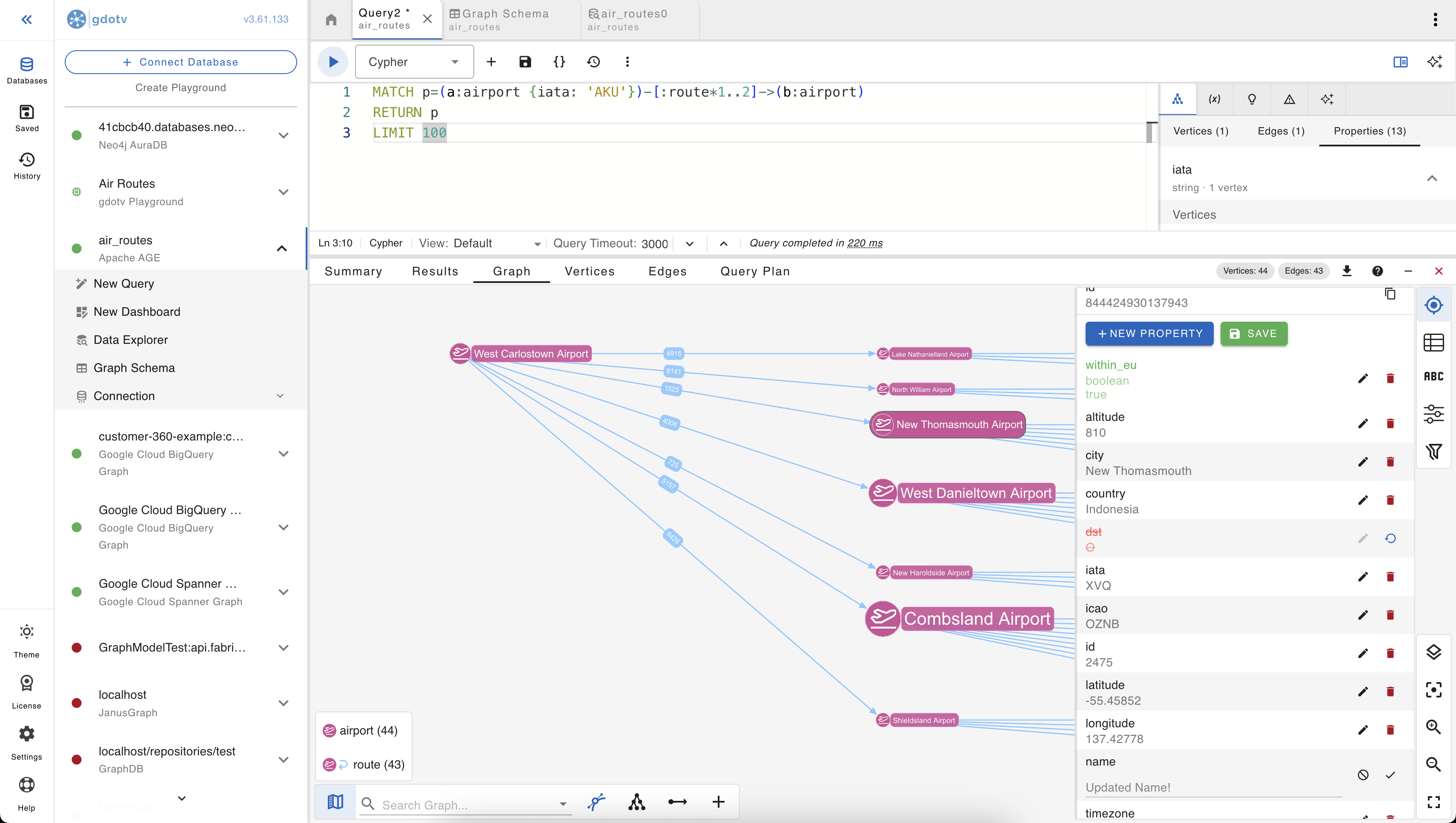
Click any vertex or edge on the canvas and the properties panel opens on the right. From there:

• Edit a property value in-place. Click the value, type the new one, save. The property panel is schema-aware, so it picks the right input control for the property’s type (numeric input for numbers, text for strings, toggle for booleans).
• Add a new property. The “New property” button adds a key/value pair to the selected element. Autocomplete on the key suggests names already used elsewhere on the same label, so you don’t accidentally end up with latitude on most vertices and Latitude on the rest.
• Delete a property with the trash icon next to it.
• Delete the vertex or edge entirely, with edge cascading on vertex deletes so you don’t end up with dangling references.

The “create” side of CRUD works the same way: a “new vertex” action drops a blank vertex onto the canvas with a label picker pre-populated from the schema, and a “new edge” action lets you connect two selected vertices, also with a schema-derived label suggestion.

Everything generates a real Cypher CREATE / SET / DELETE under the hood, run inside a transaction so a multi-property change is applied atomically.

This combination of visual exploration and visual editing is the part that’s hardest to get from any other tooling around AGE today: most graph-aware clients are read-only, and most write-capable Postgres clients don’t know how to render or write a graph. Closing that loop in a single tool is most of the reason gdotv exists.

Where to go from here

A short recap of the series:

• Part 1: Apache AGE Explained: how does it work and how does it fit in the Graph Database Landscape?. Background reading on what AGE is, how it stores graphs, and how it compares to popular alternatives.
• Part 2: Running Apache AGE: Docker Quickstart and Cloud Postgres Provider Landscape. How to actually run AGE — locally via Docker, on Azure Database for PostgreSQL or HorizonDB, on EnterpriseDB — and where it isn’t available (AWS RDS/Aurora, GCP Cloud SQL, Supabase).
• Part 3: Loading Data into Apache AGE: A Practical Guide with the Air Routes Dataset. Two loading approaches — the built-in agload and a Postgres staging-table pattern using COPY and UNWIND — with explicit attention to property type handling.
• Part 4 (this one): connecting gdotv to AGE, schema discovery, the Cypher editor, graph visualization, and interactive exploration.

If you’re picking up AGE for a real workload, the practical next steps are usually:

• Get the data right. Loading once for a tutorial is easy; loading repeatedly from changing source data is where the staging-table approach from part 3 starts paying off.
• Pick your deployment. The cloud-provider landscape from part 2 is the part that moves fastest, so verify each row against the provider’s current docs before committing.
• Get a graph-aware client in front of it. gdotv ships with a 3-week free trial that covers the full feature set described in this post against graphs of any size, including the full air routes dataset (around 3,500 airports and 20,000 routes).

Conclusion

And that’s a wrap on exploring Apache AGE! With PostgreSQL being one of the most popular databases in the world, extensions like Apache AGE help bring better visibility of graph workloads to the masses – we think that’s great.
It’s also very encouraging that this project is available at least on some (but far from all) cloud managed PostgreSQL services out there.
There are some quirks to using Apache AGE, and you should not expect native graph database performance level from it, but it also benefits from one of the most mature ecosystems in the database industry.
We strongly encourage you to check out gdotv with Apache AGE, or any other graph database you might be using!