Fill Your AWS Neptune Graph with S3 Data

Amazon Web Services. Versatile? Yes. Simple? Not always.

If you’re like most AWS users, you’re probably always looking for tips and tricks to manage your AWS data and make the most of all the services on offer. That’s why it’s super exciting that Amazon Neptune now supports calling data directly from your S3 bucket – no complex data imports necessary!

Note: You need Neptune Database 1.4.7.0 or above to load data in this way! This is being rolled out by region, and at time of writing is not available to all clusters globally yet.

Wow, nice. How does it work?

We can call data from our S3 bucket using the CALL neptune.read() function. This function reads CSV or Parquet data directly into your Neptune instance:

We’ll use gdotv to see our AWS Neptune cluster update with data from our S3 bucket in real time.

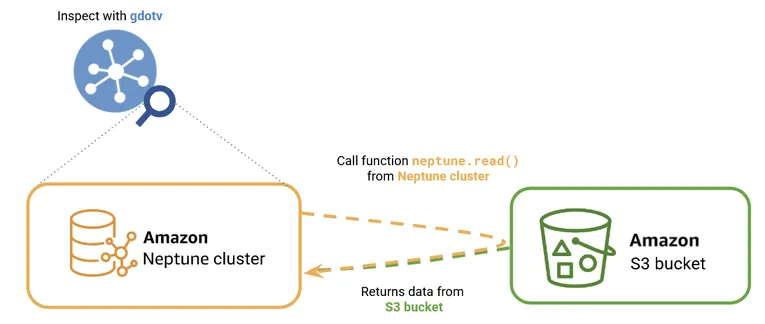
To visualize and understand our results, we’ll also connect our Neptune cluster to gdotv to get a better look at what’s happening.

Connect Your Database to gdotv

Connecting your Neptune database to gdotv is easy. All you need is the location of your database, and any credentials you might have, and you’ll be connected in seconds:

Connect to your AWS Neptune cluster in just a few seconds

You can visit our welcome portal for Amazon Neptune or watch our two-minute tutorial video, Getting Started with Amazon Neptune + gdotv to learn more..

Importing Relational Data

The next step is to choose our relational data source.

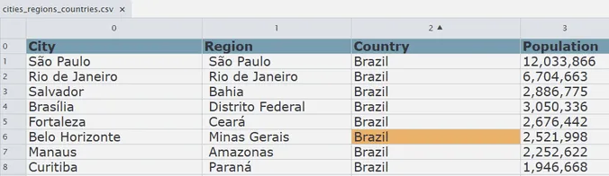
As a simple example, you can use our cities_regions_countries.csv dataset that is publicly available. It contains information on major cities within the seven largest countries in the world (India, China, the USA, Indonesia, Pakistan, Nigeria and Brazil).  Here’s an example of the function you’ll use:

A look at our relational data source, stored in our S3 bucket.

Here’s an example of the function you’ll use:

CALL neptune.read({
source: 's3://neptune-graph-import/datasets/cities_regions_countries.csv',
format: 'CSV'
})
YIELD row
MERGE (n:City {name: row.City, population:row.Population})
MERGE (r:Region {name: row.Region})  
MERGE (c:Country {name: row.Country})
MERGE (n)-[:LOCATED_IN]->(r)
MERGE (r)-[:LOCATED_IN]->(c)
RETURN n LIMIT 10

Let’s break down what this query does:

The anatomy of our query that will call data from our S3 bucket and construct a graph

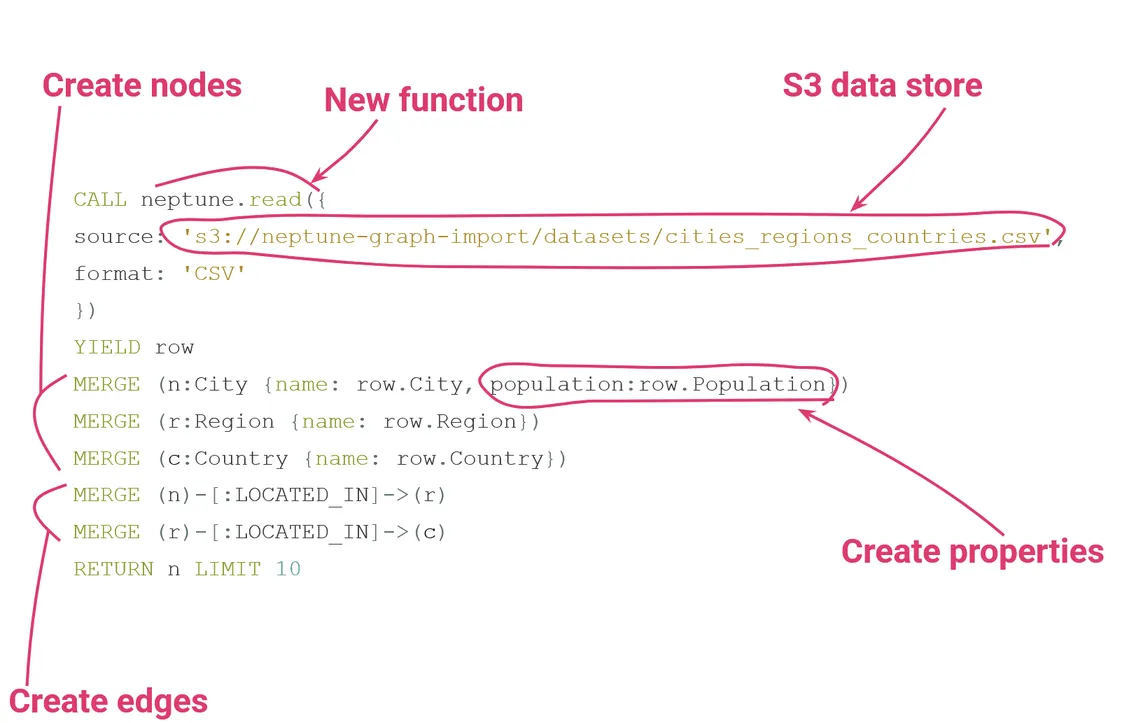
As you can see, we’re using the new neptune.read() functionality to import data from our S3 bucket.

Since that data is relational, we want to turn it into a graph form. The way we do that is by pulling each row using YIELD and creating new nodes and edges from the columns of that data using MERGE and row.[column] syntax.

Finally, we use another MERGE command to create new [:LOCATED_IN] edges.

Visualize the results!

Let’s take a look at our graph results:

MATCH p=()-[]-() RETURN p LIMIT 1000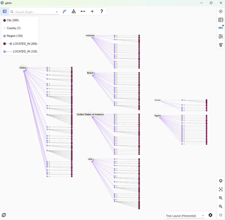

A first look at our graph, created from our relational data

As we can see, the data looks how we expect! All our City nodes are grouped according to the Region and Country nodes.

By zooming in, we see that some regions have a very high number of major cities, such as Jiangsu in China or São Paulo in Brazil:

We can identify some highly connected nodes instantly in this graph view.

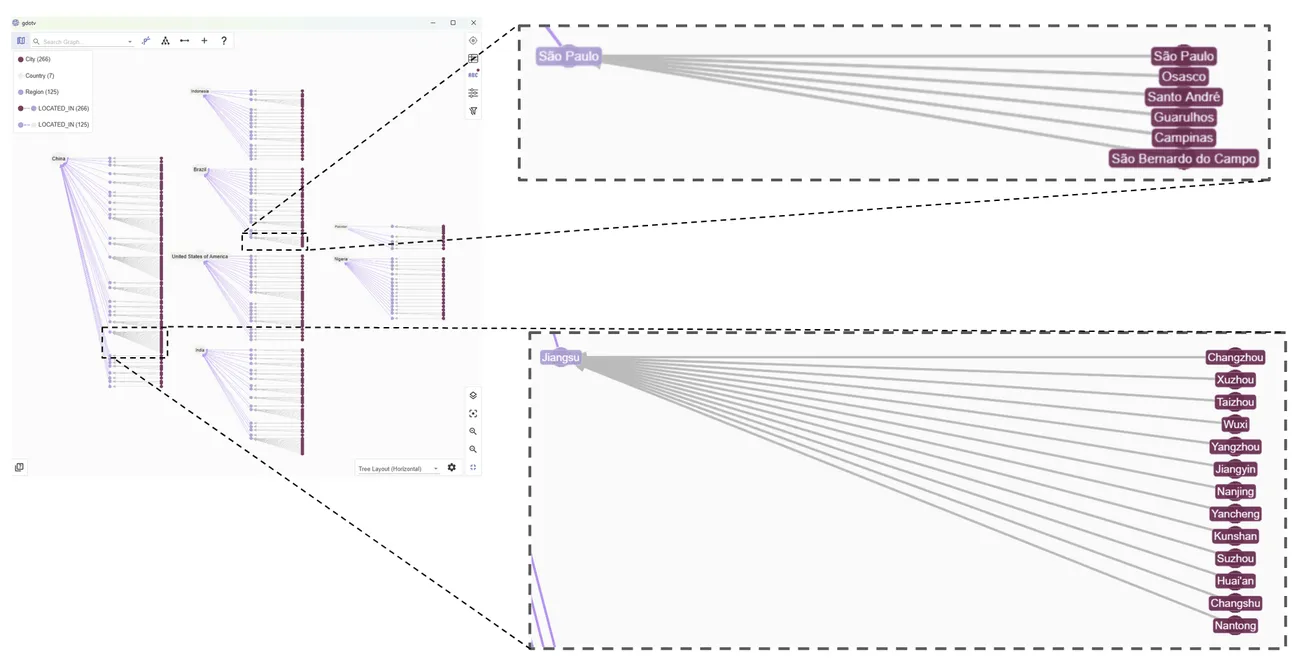
Quickly identifying highly connected regions like this is the kind of application graph visualization is ideal for — something that would be much harder to do directly from the tabular data!

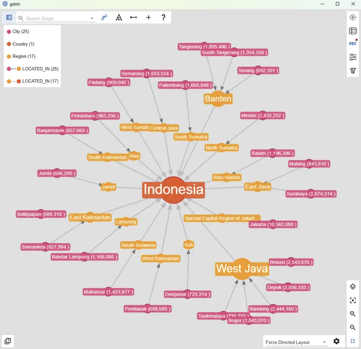
We can now take a closer look. The gdotv editor actually lets us query the graph using either Cypher or Gremlin, so lets try the following Gremlin Query to take a closer look at the node for Indonesia:

g.V().has('name', 'Indonesia').inE().outV().inE().path().limit(10000)

This lets us see at a glance, for example, that many of the biggest cities are in the West Java region!

Examining a single Country node (Indonesia) up close.

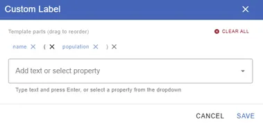
Another benefit of viewing our data in gdotv is that we are able to customize our data to look how we want.

Here, for example, we have customized the node labels to include both the name property and the population property.

A custom label created using the name and population properties, along with custom strings designating paranthesis.

Further Exploration

There we have it: a simple straightforward way to access your S3 data directly from the query editor. It’s so easy that it only takes a few lines of code, and you can visualize your data instantly within gdotv.

If you’d like more information on the neptune.read() function, check out the following AWS pages:

• [AWS Documentation] openCypher extensions in Amazon Neptune
• [AWS Documentation] Query examples using parquet
• [AWS Database Blog] Explore the new openCypher custom functions and subquery support in Amazon Neptune

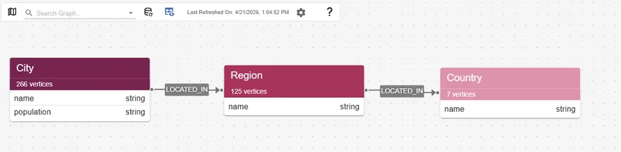
For more ways to explore your data in gdotv, you can also take a look at the Data Model view:

The data model. It has a simple form as we have used a basic relational dataset for this example. It can, however, be arbitrarily complex, depending on the structure of your data.

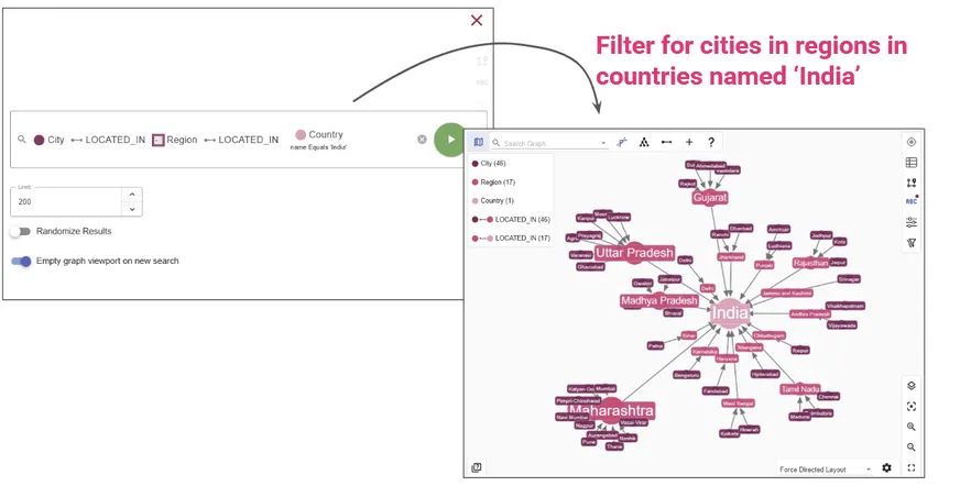
Or check out gdotv’s no-code Data Explorer to search for relationships and apply filters without writing any queries at all:

You may use the Graph Data Explorer to explore relationships in your graph.

We’d love to hear what you get up to, so let us know how you’re using gdotv to explore your relational data!