Full Steam Ahead! Fast-Tracking Your Graph Creation with Nodestream

Here at gdotv we love solutions that make building and managing graphs easier. If you read our blog, chances are that you do too! So, today, we’re turning the spotlight to Nodestream.

What’s Nodestream?

In short, Nodestream is a declarative framework for graph construction, management and analysis. It’s also an open-source community project available on GitHub and fully compatible with both Neo4j and Amazon Neptune.

In Nodestream, you define YAML configuration files that map and transform various data sources into data ingestion pipelines for your graph database.

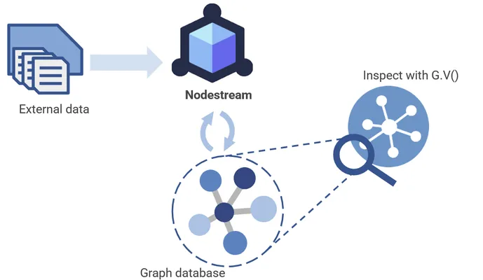
Today we want to show you just how easy it is to get started. So all aboard, because we’re going to have a little fun using Nodestream to make some train lines! At the end we’ll visualize the results in gdotv, so that you can see just how well Nodestream and gdotv pair together to give you incredible graph-based views in seconds!

Where to Get Nodestream?

Nodestream is available via the GitHub or, like any regular Python package, you can install it with pip:

pip install nodestream

Once you’ve installed Nodestream, you’re ready to get going right away.

A workspace in Nodestream is called a project, and we’re going to start by making our very first project. Thankfully, Nodestream has a built-in function to create a sample project to save us some time:

nodestream new my_project --database neptune

Running this will create a number of files in the folder /my_project.

If we explore the contents, we can see that the overall structure of your project will look something like this:

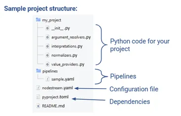
This project includes a few python scripts and a .toml file to manage your dependencies. We’ll ignore these for now. We just want to get a simple YAML-based project up and running, so we’re going to focus on the two YAML files we can see.

The first file in your root directory is the configuration file, nodestream.yaml. The second file is a sample pipeline which has also been created for you, sample.yaml, which is stored in the /pipelines folder.

The first file is the most important file to your project. That’s because the general structure of a nodestream project looks like this:

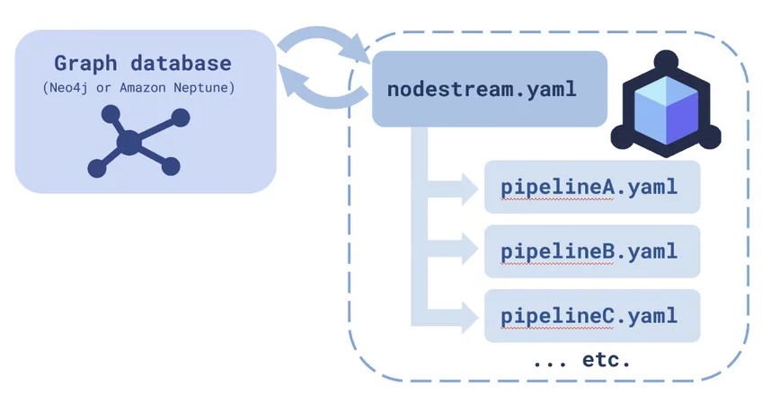
As you can see, the configuration file, nodestream.yaml, is at the center of everything. This is the file that manages all your other YAML files, which are all just a collection of pipelines, pipelineA``.yaml,pipelineB``.yaml, and so on, each carrying out its own task. We’ll show you how to configure these pipelines soon (and don’t worry – like everything else in Nodestream, it’s easy!) but first we’ll walk you through how to set up your configuration file

Another important aspect of this configuration file is that it outlines how your project will communicate with a graph database of choice – one of either Amazon Neptune or Neo4j.

Configuration

So how do we write the configuration file, nodestream.yaml? The first step is to define the scope for your project. This is essentially just a list of all the pipeline files that will be used within your project.

scopes: default: pipelines: - pipelines/sample.yaml

Now you’ve configured the pipelines within your project. As you can see, this sample project starts with just our starter pipeline file. But rest assured, we’ll set up some more soon enough!

The second function is to set up your graph database connection.

my-db: database: neptune host: https://: region: us-west-2

You have two options for your database. You can use either a Neo4j instance or an Amazon Neptune cluster.

If you’d like to use an Amazon Neptune cluster, you can use our existing guide on connecting your local environment to a Amazon Neptune cluster. Note that since we released that guide, Amazon Neptune have introduced the capability to make a Neptune cluster publicly accessible, which speeds things up quite a bit. To do this, you can follow Part 1 of the guide with a couple of changes:

• Make the Neptune instances publicly accessible.
• Turn on IAM Authentication

You may also need to install the Nodestream neptune plugin for this two work:

pip install -q pyyaml nodestream-plugin-neptune

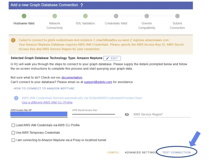
Connecting to your Amazon Neptune or Neo4j database with gdotv takes only a few seconds. You just need to click New Database Connection, enter the location of your database along with your authentication credentials, and hit Test Connection:

Managing Your Pipelines

Before we get onto actually writing a pipeline for our sample project, or constructing a custom one, there are a couple extra utility functions for pipeline management that it’s good to know. These are for individual projects, so remember to cd into your project before you use them!

Since Nodestream follows such a simple structure, adding and removing pipelines is straightforward. You just adjust your available .yaml files, and edit the configuration file accordingly.

But wouldn’t it be nice if we could speed up the process? That’s why Nodestream includes a few time-savers…

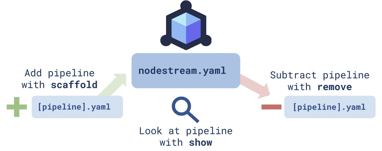
Use the command remove to remove a pipeline:

nodestream remove default sample

^default corresponds to the ‘default’ scope

We can also use the command scaffold toadd a pipeline:

nodestream scaffold new_pipeline

For one final handy trick, you can review the status of your project using:

nodestream show

Here’s a summary of each command:

And that’s it! We’re ready to start streaming some nodes.

Pipeline Introduction

Okay, so we’ve set up the basics of our project. We’ve got our configuration file (nodestream.yaml) established with a graph database connection and containing at least one pipeline. With our structure now in place, we just need to decide what our pipeline will actually do.

The default pipeline, sample``.yaml, creates a set of numbered nodes. You can find a description of that basic code here if you’re interested, but we’re going to skip straight ahead to making a graph out of some actual data.

Nodestream does provide a simple data-based example already. If you’d like to follow that, you can follow the instructions in Managing Your Project and Create a New Pipeline to replace the default sample file with a new file, org-chart``.yaml. You’ll also have to create the accompanying employees.csv file provided in the tutorial.

We’re going to make our own data-based example, but before we do that, let’s crack open the example given, org-chart``.yaml, and take a look.

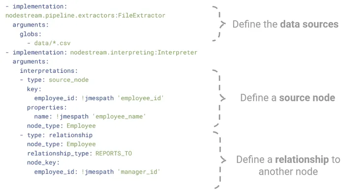
The first part of the code uses the FileExtractor to (as the name might suggest!) extract data from some files. It looks for any data of the form data/*.csv. It tells the script that it will be fed a series of strings that correspond to input files.

The second part lets the code know how to interpret the input data as a series of nodes and relationships. It generates nodes with a key based on the employee_idcolumn and creates a single property (name) from the employee_name column. It then interprets a relationship between that node and another Employee node based on the manager_id column.

We’ll spend more time looking at the precise syntax in the next example, but hopefully you get the idea. The result for this sample graph should look something like this:

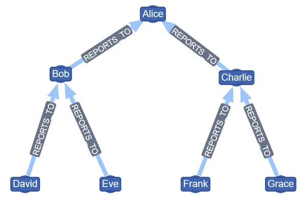
We’ve now moved through all the basic tutorials on the Nodestream documentation. It’s time to move onto the next step, which is creating an entirely new graph of our own…

Creating a new pipeline

Since gdotv is based in Scotland, and we love to travel, we’ve chosen to use Nodestream to process some transport data from the Scottish Highlands & Islands. We’ve focused on public transport links in particular, things like: train or bus routes, or ferry routes over water. At the end, we’re going to aim to turn the result into a useful map.

We’ll map out various station nodes, which could be connected by train, bus or ferry edges. That means our data model will look something like this:

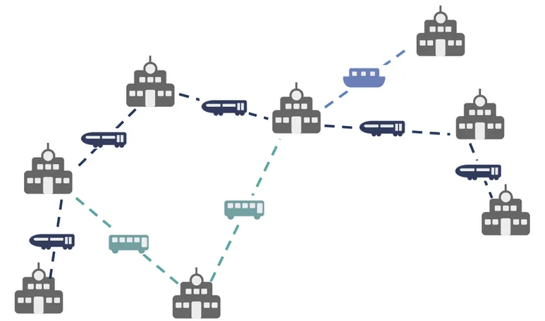
Of course public transport data is typically publicly available, so you’re free to map a different region if you like, but we expect you’d rather not transcribe any routes by hand! To save you time you can grab a copy of our precompiled files for northern Scotland via our GitHub.

Inside you’ll find both our raw data and our code for this data. You can find them each in the /data and /pipelines folders, respectively.

The data falls into two types, divided by nodes and edges. All the stations (nodes) are found in one store: the stations.csv file. The routes (edges) are distributed over a number of files depending on the route type, designated by route_*.csv.

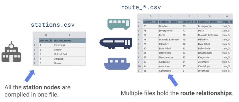
Our first pipeline, scotland_chart.yaml, is responsible for extracting all our nodes from the stations.csv file.

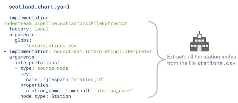
Just as before, we define the location of our input data. Next, we can see that we scan this file looking for source nodes.

One important trait of Nodestream is that the source node is always the center point of any piece of data being ingested. Everything starts from a source node, which should either reference an existing node, or a new node to be created. If a new data ingestion references a source node that has already been created, then the old and new data will be merged – or replaced, in the case of conflicts!. So while you probably will want to reference existing nodes, you should be careful how you handle them.

We then extract data from columns using the !jmespath tag, which extracts JSON data. Just as before, we assign to this source node a key (unique identifier) and a node_type (‘Station’). You might wonder why the key has the subkey name. That’s because, interestingly, you can define multiple keys to make a composite key! We also use the properties key to assign properties based on the station_name column.

Now we’ll take a look at our second pipeline file, scotland_chart.yaml, which extracts all the relationships.

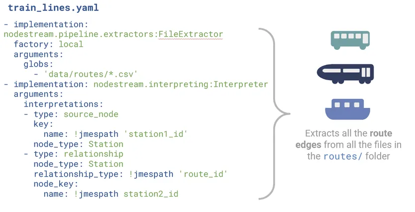
We can see that once again we start from the source_node. Again, no matter what data we’re ingesting, we always define the source_node. But this time we don’t need to define any properties, like the station name, for the node. That’s because the station name has already been defined in the previous pipeline! Last time (in the employees example) we created the source node along with the relationship. This time, we’re referencing an existing node. All we need is the key to identify the correct node, which we extract from the station1_id column.

We could, however, assign any new properties we like. For example, we could choose to add information about the district of the station using an is_in label, or accessibility information via a has_wheelchair_access label. We can add this information in any database we like, without worrying about updating all of them at once. That’s because Nodestream handles data merging for us.

Now that we’ve defined the source node, we can define the rest of the relationship. We use another !jmespath to define the relationship_type by the route type, meaning that we’ll now define multiple types of edges (the previous example had only one: reports_to). We also define the target node by its node_type and node_key.

Visualizing the data with gdotv

Okay – hopefully Nodestream has had no issue turning this into graph data, so let’s fire up gdotv and have a look at the final result. You should be able to see your graph instantly:

(Revisit the Configuration step above if you’d like to review how to get connected with gdotv!)

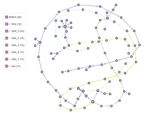
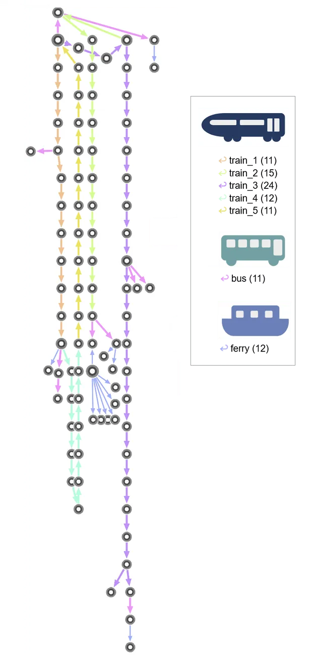
Not bad! We can see all our routes winding around and tangled up in each other. By default gdotv loads graphs in the Force-Directed Layout. This is great for node + edge spacing, so you can get a good feel for the shape of the data. However the location of nodes themselves is pretty random, which probably isn’t ideal for public transport data. Since in real life we would physically move along these lines, you’d like this kind of data to conserve some sense of direction.

One option is that instead, you could use Tree Layout (Vertical) or Tree Layout (Horizontal) to get a more recognizable train map.

You can turn on labels and zoom in to get a closer look at your data and browse interactively:

Alternatively, you can play with our customization options to create stylistic, static charts:

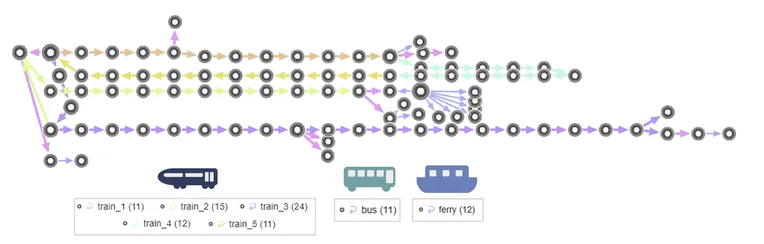
Another option is that you can manually manipulate the nodes to represent their physical locations. Remember that you have full control of the node, edge and labeling design. Add a few lines, and you’ve got a geographical train map in seconds!:

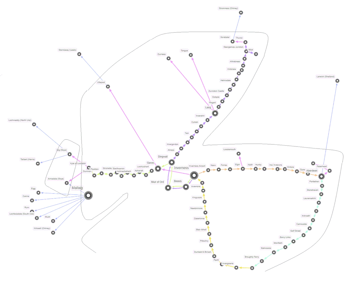
Compare our map to the official ScotRail map to see how we did!

There are also several more layout and customization options you can explore within the gdotv interface. You’ll find some of them suit this particular dataset better than others – but play around and make up your own mind!

Isn’t that amazing? We’ve gone from simple spreadsheets to birds-eye graph views of interconnected data in seconds. That’s the power of Nodestream and gdotv – a combination we certainly recommend.

Conclusion

There we have it! You can see just how accessible graph data exploration becomes with Nodestream. By lowering the barriers to entry, it opens the door for developers of all levels to build pipelines, connect data, and visualize results with ease – especially when paired with gdotv.

Our Scotland transport example is just the beginning—wherever your data lives, Nodestream is ready to handle it. Why don’t you check out the links below, and learn more?

• Welcome to Nodestream
• Basic tutorials
• Nodestream GitHub