Build Your First Recommendation System with BigQuery Graph

We’re excited to share that gdotv now supports BigQuery Graph – Google’s native graph capability built directly into BigQuery. That means you can model, query, and visualize connected data right within your existing BigQuery environment, without managing a separate graph database. To learn more details on how BigQuery graph pairs with gdotv, check out the dedicated BigQuery landing page.

In this post, we’ll walk through Google’s own BigQuery Graph codelab demo, which builds a Customer 360 view and a product recommendation engine for a fictional retail company called Cymbal Pets.

Along the way, we’ll show you how gdotv lets you instantly visualize the results of your graph queries – turning raw SQL output into rich, interactive graph visualizations.

Here’s what we’ll cover:

•   Setting up the dataset in BigQuery
•   Defining and populating a the property graph
•   Writing some basic graph queries using Google SQL
•   Visualizing customer purchase history and product recommendations in gdotv

Let’s get into it!

Getting Set Up with BigQuery Graph & gdotv

Here’s an overview of the approach we want to use:

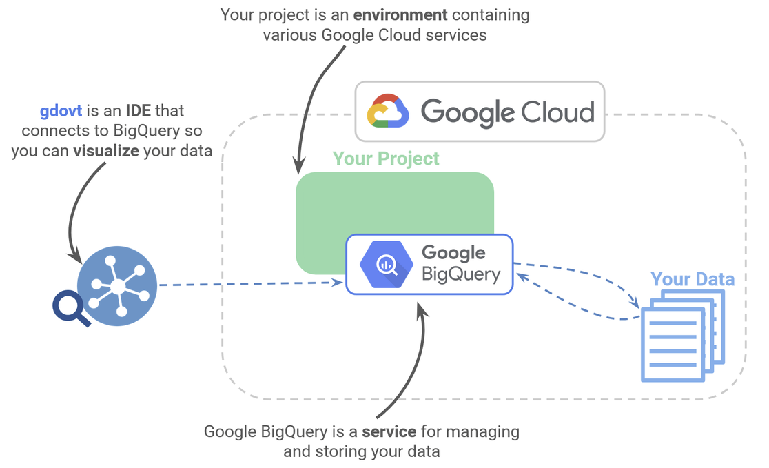
An overview of how we manage our Google Cloud data with BigQuery and visualize with gdotv.

We’ll set up a Google Cloud project, and then use the Google BigQuery service to manage our data. We’ll use the new functionality, Google BigQuery Graph, to set up a property graph. Then we’ll visualize the results in gdotv.

BigQuery Graph doesn’t require any additional infrastructure. It lives natively inside BigQuery Studio, and BigQuery service itself comes with your Google Cloud Project. So, as long as you have a Google Cloud project with billing enabled, you’re ready to go! If you don’t have a project already running, you can follow the instructions here to set one up.

From here, much of your setup will take place in the Google Cloud Console. The Google Cloud Console is a great place to manage your project. For our purposes, follow Step 2 – Before You Begin of the codelab demo. This will use your Google Cloud Console to active the Cloud shell and confirm your settings.

All you need now is gdotv to tackle the data visualization. Head over to the download portal to install it if you haven’t already. We’ll use gdotv to connect to the BigQuery service and inspect our data.

Connecting to BigQuery from gdotv is quick and straightforward. Once you’ve navigated to Connect a Database on the landing page, you can point gdotv at your BigQuery project. All you need is the location of your project. Within seconds, you’ll be ready to start visualizing your graph data. No complex configuration required!

Connect gdotv to your Google BigQuery Graph in just a few seconds.

The Data Model: Cymbal Pets

Before we dive into queries, let’s take a look at the graph schema we’ll be building. The Cymbal Pets dataset models a retail company’s operations, with four main node types and several relationships connecting them.

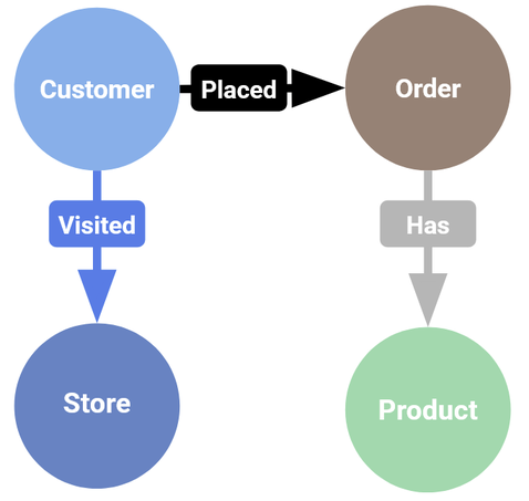
A basic overview of our data model.

Node types:

•   Customer – individual shoppers
•   Orders – purchase records with dates, payment methods, and shipping info
•   Products – items for sale, each with an embedding vector for semantic similarity search
•   Stores – physical store locations

Edge types:

•   Placed – connects a Customer to an Order
•   Has – connects an Order to a Product
•   Visited – connects a Customer to a Store via an order

Defining the Schema and Loading Data

Creating the Dataset and Tables

Start by creating the cymbal_pets_demo dataset and its tables in the BigQuery SQL Editor:
CREATE SCHEMA IF NOT EXISTS cymbal_pets_demo;

You’ll then create six tables:
customers, products, orders, order_items, stores, and co_related_products_for_angelica.

Here’s an example of the tables we’ll create. Note that we found you needed to remove the PARTITION BY and CLUSTER BY lines on the order schema, which includes a vector embedding column we’ll use later for recommendations:

CREATE TABLE IF NOT EXISTS cymbal_pets_demo.order_items
(
  order_id INT64,
  product_id INT64,
  order_item_id INT64,
  quantity INT64,
  price FLOAT64,
  PRIMARY KEY (order_id, product_id, order_item_id) NOT ENFORCED
)
CLUSTER BY order_item_id;

CREATE TABLE IF NOT EXISTS cymbal_pets_demo.products
(
  product_id INT64,
  product_name STRING,
  brand STRING,
  category STRING,
  subcategory INT64,
  animal_type INT64,
  search_keywords INT64,
  price FLOAT64,
  description STRING,
  inventory_level INT64,
  supplier_id INT64,
  average_rating FLOAT64,
  uri STRING,
  embedding ARRAY,
  PRIMARY KEY (product_id) NOT ENFORCED
)
CLUSTER BY product_id;

CREATE TABLE IF NOT EXISTS cymbal_pets_demo.orders
(
  customer_id INT64,
  order_id INT64,
  shipping_address_city STRING,
  store_id INT64,
  order_date DATE,
  order_type STRING,
  payment_method STRING,
  PRIMARY KEY (order_id) NOT ENFORCED
)

CREATE TABLE IF NOT EXISTS cymbal_pets_demo.stores
(
  store_id INT64,
  store_name STRING,
  address_state STRING,
  address_city STRING,
  latitude FLOAT64,
  longitude FLOAT64,
  opening_hours STRUCT,
  manager_id INT64,
  PRIMARY KEY (store_id) NOT ENFORCED
)
CLUSTER BY store_id;

CREATE TABLE IF NOT EXISTS cymbal_pets_demo.customers
(
  customer_id INT64,
  first_name STRING,
  last_name STRING,
  email STRING,
  gender STRING,
  address_city STRING,
  address_state STRING,
  loyalty_member BOOL,
  PRIMARY KEY (customer_id) NOT ENFORCED
)
CLUSTER BY customer_id;

CREATE TABLE IF NOT EXISTS cymbal_pets_demo.co_related_products_for_angelica
(
  angelica_product_id INT64,
  other_product_id INT64,
  co_purchase_count INT64
);

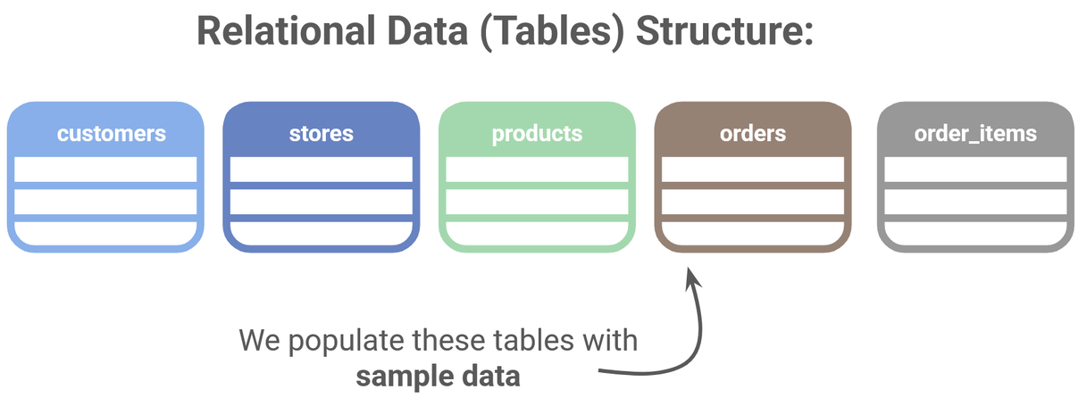
The structure of our relational data store.

Loading Sample Data

Load the sample data directly from Google Cloud Storage using LOAD DATA statements as defined in Step 4 – Load the Data of the demo:

LOAD DATA INTO `cymbal_pets_demo.customers`
FROM FILES (
    format = 'AVRO',
    uris = ['gs://sample-data-and-media/cymbal-pets/tables/customers/*.avro'],
    enable_logical_types = true
);

Repeat this for the orders, order_items, products, and stores tables. Once complete, you should see row counts confirming successful data loading in each table.

Creating the Property Graph

With the data in place, the next step is to define the Property Graph itself. This tells BigQuery which tables represent nodes and which represent edges – and how they connect to each other.

Our approach closely follows Step 5 – Create the Property Graph of the demo.

CREATE OR REPLACE PROPERTY GRAPH cymbal_pets_demo.PetsOrderGraph
NODE TABLES (
  cymbal_pets_demo.customers KEY(customer_id) LABEL Customer,
  cymbal_pets_demo.products KEY(product_id) LABEL Product,
  cymbal_pets_demo.stores KEY(store_id) LABEL Store,
  cymbal_pets_demo.orders KEY(order_id) LABEL anOrder
)
EDGE TABLES (
  cymbal_pets_demo.orders as customer_to_store_edge
    KEY (order_id)
    SOURCE KEY (customer_id) references customers(customer_id)
    DESTINATION KEY (store_id) references stores(store_id)
    LABEL Visited
    PROPERTIES ALL COLUMNS,

  cymbal_pets_demo.order_items
    KEY (order_item_id)
    SOURCE KEY (order_id) references orders(order_id)
    DESTINATION KEY (product_id) references products(product_id)
    LABEL Has
    PROPERTIES ALL COLUMNS,

  cymbal_pets_demo.orders as customer_to_orders_edge
    KEY (order_id)
    SOURCE KEY (customer_id) references customers(customer_id)
    DESTINATION KEY (order_id) references orders(order_id)
    LABEL Placed
    PROPERTIES ALL COLUMNS,

  cymbal_pets_demo.co_related_products_for_angelica
    KEY (angelica_product_id)
    SOURCE KEY (angelica_product_id) references products(product_id)
    DESTINATION KEY (other_product_id) references products(product_id)
    LABEL BoughtTogether
    PROPERTIES ALL COLUMNS
);

This diagram illustrates how data from our various relational databases are used to build our graph. You can see, for example, that the order_items table is used to build the [Has] edge while also pulling data from the orders and products tables! This illustrates the dynamic way BigQuery can be used to construct graphs from relational data. One of the great things about BigQuery Graph is that it lets you match patterns across multiple tables in this way.

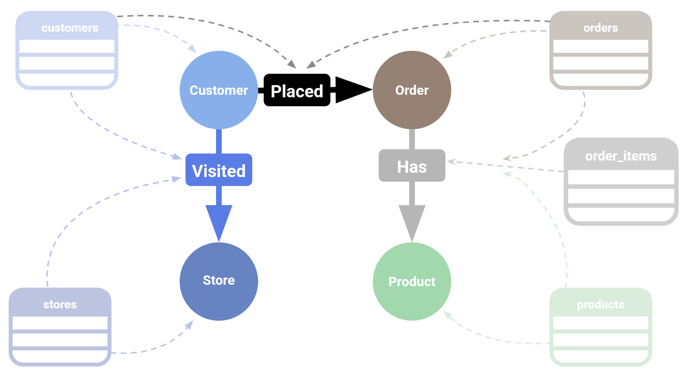
How our relational data will map to our graph data.

The result is a simple but intuitive model that makes it easy to see what’s going on.

Assuming that you have connected gdotv to your BigQuery project, you see this data model for yourself by clicking Graph Schema to see this schema laid out visually – and it updates in real time as your data evolves.

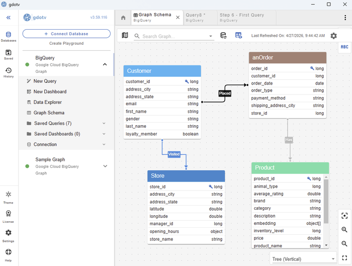
The data model for our BigQuery graph as visualized within gdotv.

Visualizing Customer Purchase History in gdotv

Let’s look at the data. Of course we could just run a simple sample query to graph the first 1000 relationships we find:

GRAPH cymbal_pets_demo.PetsOrderGraph MATCH (s)-[r]->(e) RETURN TO_JSON(s) as s, TO_JSON(r) as r, TO_JSON(e) as e LIMIT 1000

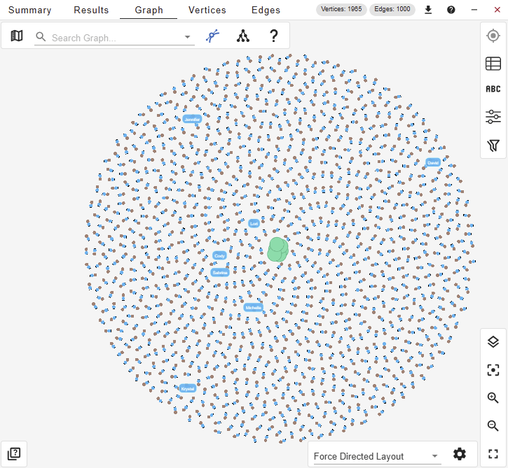
The first thousand relationships pulled randomly from our graph.

But this is a big dataset, so just graphing random relationships isn’t very informative. Let’s try something more sophisticated instead.

Following Step 6 – Visualize Purchase History of all customers of the demo, we start with a broad overview. Imagine Cymbal Pets wants to see all customers and their recent purchases in a single visualization.

Let’s try

GRAPH cymbal_pets_demo.PetsOrderGraph
  # finds the customer node and then finds all
  # the Orders nodes that are connected to that customer through the
  # Placed relationship
  MATCH (customer:Customer)-[placed:Placed]->(ordr:anOrder)-[has:Has]->(product:Product)
  # filters the Orders nodes to only include those where the
  # order_date is within the last 3 months.
  WHERE ordr.order_date >= date('2024-11-27')
  # # This line finds all the Products nodes that are connected to the
  # # filtered Orders nodes through the Has relationship.
  MATCH p=(customer:Customer)-[placed:Placed]->(ordr:anOrder)-[has:Has]->(product:Product)
  LIMIT 400
  RETURN
    TO_JSON(p) as paths

The TO_JSON(p) output is exactly what gdotv needs to render the results as an interactive graph. Once you paste the output into gdotv, you’ll immediately see the network of customers, orders, and products laid out visually – no additional configuration needed.

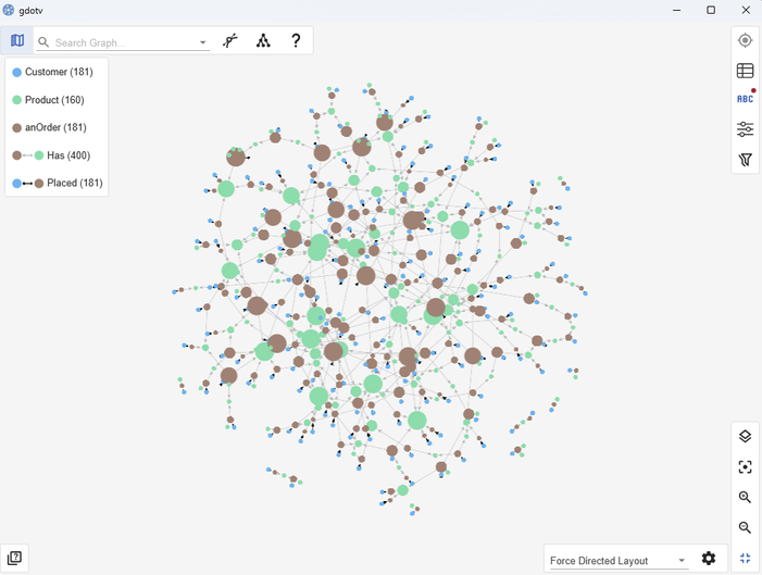
Relationships showing a Customer who has placed an Order that contains a Product.

Another great way to explore the data would be to use gdotv’s Graph Data Explorer – a no-code environment that lets you click into nodes, apply filters, and drill down into individual properties without writing a single line of additional code.

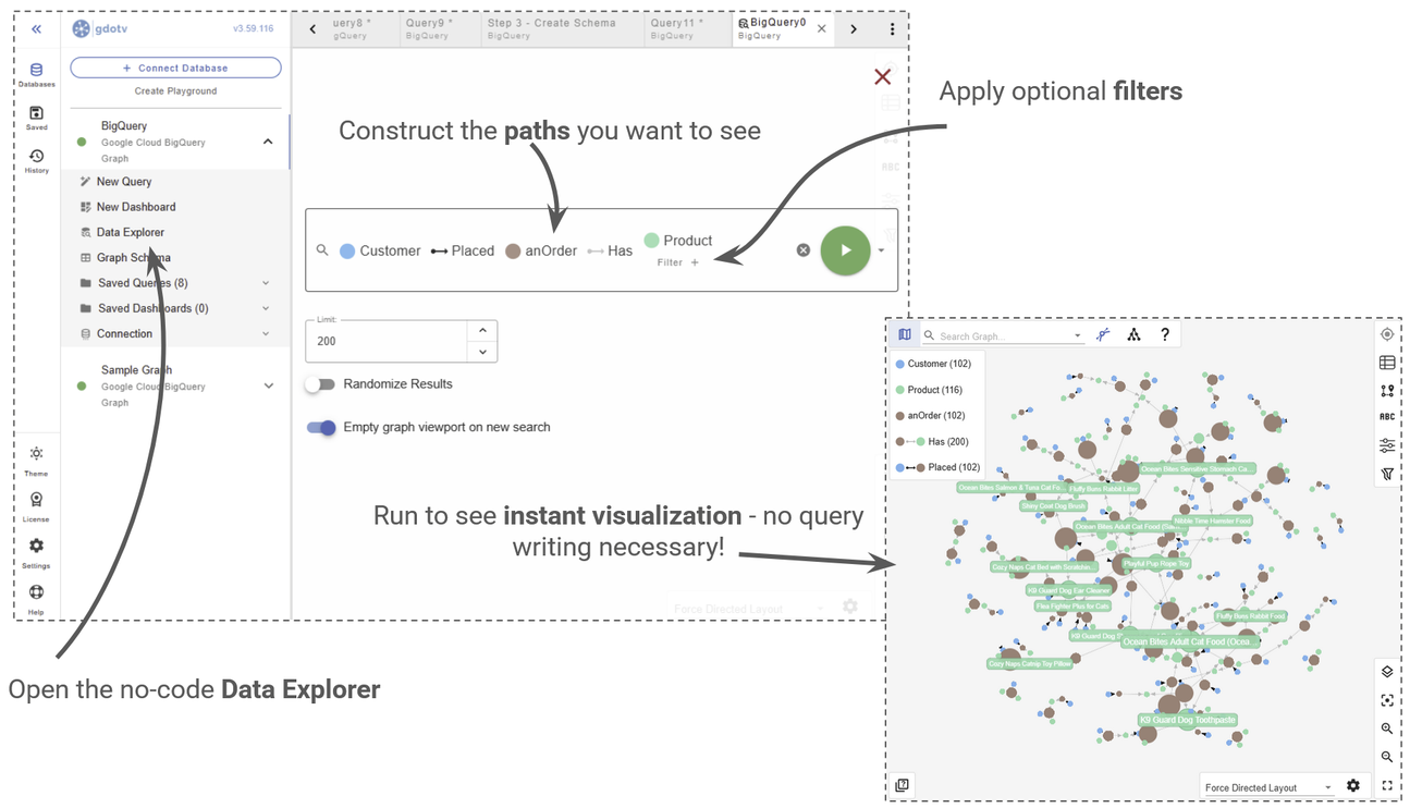
We can explore our graph data without code using the Graph Data Explorer.

A Closer Look: Angelica Russell

Now let’s take a closer look at a specific customer, as in Step 7 – Visualize Purchase History of Angelica. Cymbal Pets wants to understand Angelica Russell’s recent purchase behaviour and which stores she visited. This query captures both:

GRAPH cymbal_pets_demo.PetsOrderGraph
  # finds the customer node with the name "Angelica Russell" and then finds all
  # the Orders nodes that are connected to that customer through the
  # Placed relationship and all the Products nodes that are connected to the
  # filtered Orders nodes through the Has relationship.
   MATCH p=(customer:Customer {first_name: 'Angelica', last_name: 'Russell'})-[placed:Placed]->(ordr:anOrder)-[has:Has]->(product:Product)
  # filters the Orders nodes to only include those where the
  # order_date is within the last 3 months.
  WHERE ordr.order_date >= date('2024-11-27')
  # finds the Stores nodes where Angelica placed order from
  MATCH p2=(customer)-[visited:Visited]->(store:Store)
  RETURN
    TO_JSON(p) as path, TO_JSON(p2) as path2

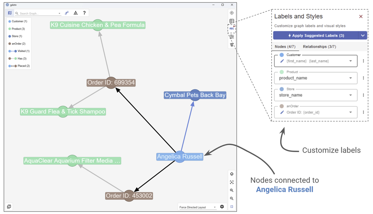
Zooming in on the purchase history of a specific user.

In gdotv, you’ll see Angelica at the centre of her own subgraph – connected to the orders she placed, the products she purchased, and the stores she visited. You can click on any node or edge to see its full list of properties in the object view, or switch to the table view to see everything in a structured format.

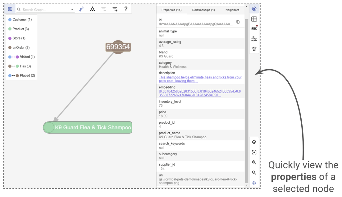
Examine the properties of a certain node up close.

You can also use gdotv’s customization options to style the graph however you like – changing node colours by label type, adjusting edge labels, or switching between layout algorithms to get the clearest possible picture of the data.

Visualizing Customer Purchase History in gdotv

Subsequent steps of the demo discuss how the results of a vector search can be used to construct a new boughtTogether edge. It then shows how this can be used to construct a product recommendation suggestion algorithm based on similarity indexes.

You can see below how what this new edge looks like in gdotv:

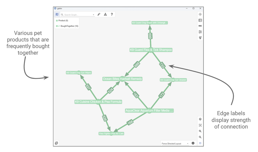
A vector search can produce new insights that can be used to construct a ‘boughtTogether’ edge.

You can also return to a specific customer, like Angelica, to see what kinds of products would be suggested based on her purchase history:

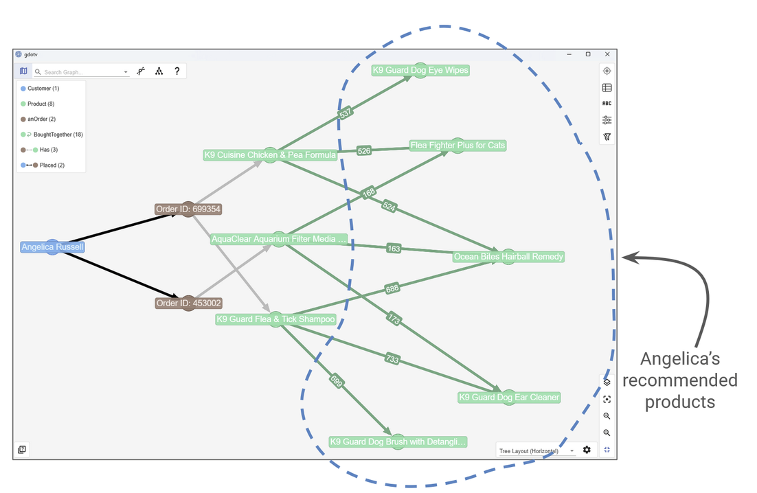
We use the ‘boughtTogether’ edge to generate product recommendations.

You can also revisit the Graph Schema to see the creation of this new edge:

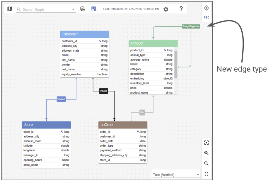
The Data Model has been updated to show the new edge.

And, of course, there will always be some situations where you just want to access your data without visualization. You can always use gdotv to produce results in tabular form too!

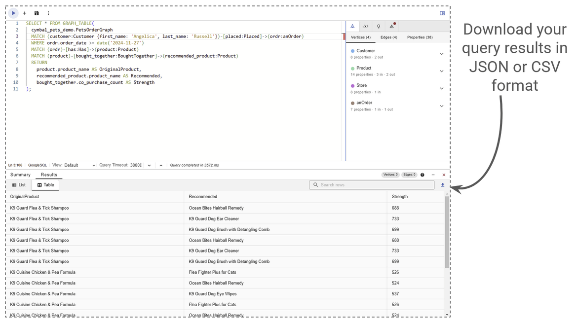
You can always export your results as raw data.

Getting Set Up with BigQuery Graph & gdotv

In this post, we’ve seen how BigQuery Graph brings native graph capabilities to one of the world’s most popular data warehouses. We built a full Customer 360 and recommendation pipeline for Cymbal Pets, and we’ve seen how gdotv makes it effortless to visualize the results.

gdotv is compatible with just about any graph on the marketplace – and BigQuery Graph is a fantastic addition to the ecosystem. Whether you’re building customer intelligence tools, recommendation systems, or just trying to understand the shape of your connected data, this pairing gives you the best of both worlds: the familiar power of SQL and the visual clarity of graph exploration. Learn more about it here.

Get in touch if you enjoyed this demo!